PICUP Solving Resistor Networks JavaScript Simulation Applet HTML5

Breadcrumbs

About

1instructorguide

These exercises are designed to get students started on using computers to solve systems of linear equations. Students should have some experience in an appropriate computational package before attempting this. Mathematica is a very good choice of tools for this exercise, closely followed by Python/numpy and MatLab. C/C++ also works, with appropriate libraries. The systems of equations we’ll be using come from resistor networks typical of a second-semester physics course, but the same techniques can be used for any system of linear equations regardless of their source.

Being able to solve systems of equations is an important computational skill, with applications in everything from mechanical engineering to quantum physics. For small systems of equations it is fairly simple to solve the systems algebraically, but for large complex systems it’s important to be able to solve them numerically using computers.

2theory

We first express the system of equations as a single matrix equation,

\begin{matrix} (1) & M x = b \end{matrix}

Since there are as many equations (rows in $M$ ) as there are variables (columns in $M$ ), $M$ will be a square matrix. If there is a solution to this set of equations, then there will exist another matrix $M^{- 1}$ such that $M^{- 1} M = I$ , where $I$ is the identity matrix. In that case,

\begin{matrix} (2) & M^{- 1} M x = M^{- 1} b \end{matrix}

\begin{matrix} (3) & I x = x = M^{- 1} b \end{matrix}

There are algorithmic methods for finding $M^{- 1}$ (and thus $x$ ; in our case we’ll be using standard libraries to calculate this matrix and the corresponding solution. One standard method is to have the computer calculate $M^{- 1}$ directly using an “invert()” function, and then multiply that inverse matrix by $b$ to obtain $x$ .

Most computational packages that have the ability to calculate $M^{- 1}$ also have an additional function, often called “solve()”, that takes care of the multiplication as well, and gives the user $x$ directly.

For more information about how these functions work, see Numerical Recipes in C by Flannery, Teukolsky, Press, and Vetterling, or similar text.

3exercises

Exercise 1: Introductory Problem

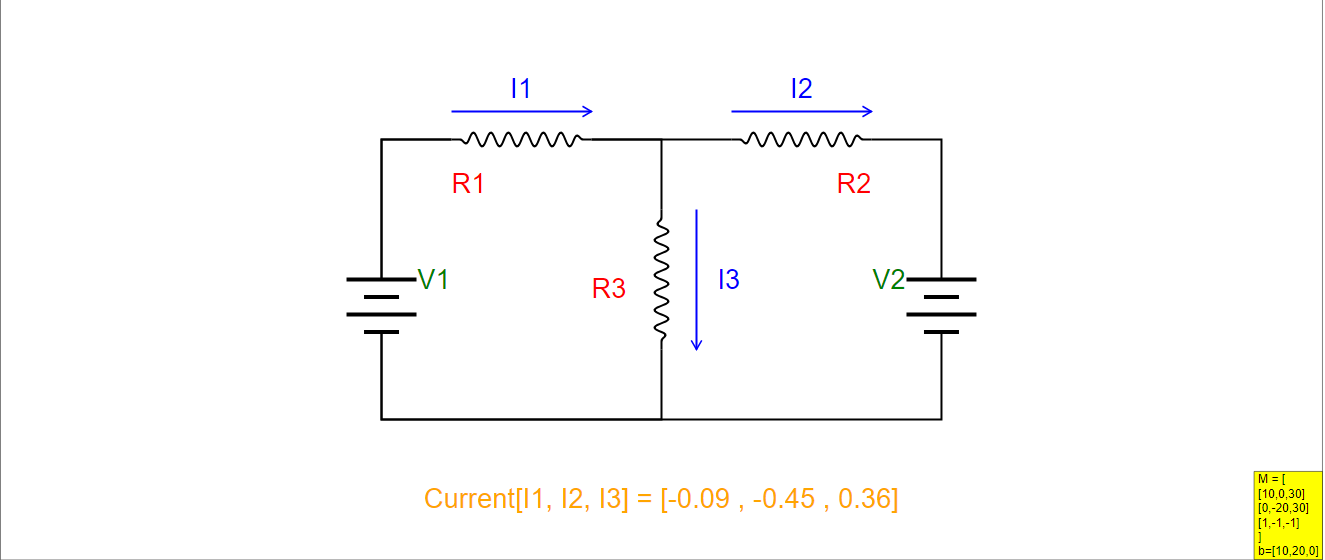
Consider the network of resistors and batteries shown in the first figure below.

There are three unknowns in that circuit, $I_{1}$ , $I_{2}$ , and $I_{3}$ . We can solve for these unknowns by building a system of equations using Kirchhoff’s Laws:

The sum of voltages around any loop is zero.
The sum of currents at any junction is zero.

Applying the voltage law to the left-hand loop, we get

\begin{matrix} (4) & V_{1} - I_{1} R_{1} - I_{3} R_{3} = 0 \end{matrix}

From the right-hand loop, we get

\begin{matrix} (5) & V_{2} + I_{2} R_{2} - I_{3} R_{3} = 0 \end{matrix}

We need one more equation, for which we can use the junction at top center and the current law:

\begin{matrix} (6) & I_{1} - I_{2} - I_{3} = 0 \end{matrix}

We now have the requisite three independent equations, which we can solve using methods learned in high-school algebra.

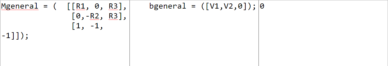
There’s another way of solving this, using matrix methods. First, rewrite the equations just a bit.

\begin{aligned} (7) & R_{1} I_{1} + 0 I_{3} + R_{3} I_{3} & = & V_{1} \\ (8) & 0 I_{1} - R_{2} I_{2} + R_{3} I_{3} & = & V_{2} \\ (9) & I_{1} - I_{2} - I_{3} & = & 0 \end{aligned}

And now we can see that this can be written as a matrix equation!

\begin{matrix} (10) & [\begin{matrix} R_{1} & 0 & R_{3} \\ 0 & - R_{2} & R_{3} \\ 1 & - 1 & - 1 \end{matrix}] [\begin{matrix} I_{1} \\ I_{2} \\ I_{3} \end{matrix}] = [\begin{matrix} V_{1} \\ V_{2} \\ 0 \end{matrix}] \end{matrix}

This matrix equation,

\begin{matrix} (11) & M x = b \end{matrix}

has solution

\begin{matrix} (12) & x = M^{- 1} b \end{matrix}

where $M^{- 1}$ is the inverse of $M$ . Most computational packages have built-in capability for inverting matrices.

ASSIGNMENT

By carrying out the matrix multiplication explicitly, show that the matrix equation above reduces to the system of equations from which it is derived.
Use a matrix-solving package to find the currents.
Check your answers by substituting the currents into the equations and verifying that they are solutions.

Exercise 2: More complicated problem

The resistor network below is perhaps a bit more challenging.

ASSIGNMENT

Write a system of equations that can be used to solve for the currents in the circuit above.
Re-write the system of equations from part 1 of this assignment as a matrix equation.
Use a matrix-solving package to find the currents.
Check your answers: do the values of currents you found solve the equations with which you started?
You may notice something interesting if you compare your solution here to your solution for exercise 1. (Assuming the same values of $R$ and $V$ were used in both exercises.) Explain why this happened.

Unless your instructor provides you with other values, assume each voltage source and each resistor has a value $10 \times$ its identifying number. (i.e. $V_{2} = 20$ V, $R_{3} = 30 Ω$ .)

Assignment

1) By carrying out the matrix multiplication explicitly, show that the matrix equation above reduces to the system of equations from which it is derived.
2) Use a matrix-solving package to find the currents.
3) Check your answers by substituting the currents into the equations and verifying that they are solutions.

resistorpy

'''

resistor.py

Eric Ayars

June 2016

A demonstration program for solving a system of linear equations using Python.

'''

import numpy as np

# Start by getting the values of R and V

R1 = float(input("R1 = "))

R2 = float(input("R2 = "))

R3 = float(input("R3 = "))

V1 = float(input("V1 = "))

V2 = float(input("V2 = "))

# Use these values to build the matrix M. Note that this matrix

# will vary depending on the equation set selected to solve the

# problem: here I use the equations from the PICUP webpage.

# Here is the matrix M:

M = np.array([ [R1, 0, R3],

[0,-R2, R3],

[1, -1, -1] ])

# here is the right-hand-side b:

b = np.array([V1,V2,0])

# And this is all it takes to get a solution:

x = np.linalg.solve(M,b)

# show the result.

print(x)

# The result is an array of currents:

# [-0.09090909 -0.45454545 0.36363636]

# The first one is I_1, the second is I_2, etc.

Translations

Code	Language		Translator	Run

Credits

Fremont Teng; Loo Kang Wee

Overview

This document provides a briefing on the "PICUP Solving Resistor Networks JavaScript Simulation Applet HTML5" resource from Open Educational Resources / Open Source Physics @ Singapore. This resource offers an interactive tool and exercises designed to help students learn how to use computational methods, specifically matrix algebra, to solve systems of linear equations derived from resistor networks. The content is primarily aimed at a second-semester physics course level but emphasizes the broader applicability of these techniques to various fields.

Main Themes

Computational Problem Solving: The central theme is using computers to solve systems of linear equations. The resource highlights that while algebraic methods are suitable for small systems, numerical methods implemented on computers become essential for larger, more complex systems.

"Being able to solve systems of equations is an important computational skill, with applications in everything from mechanical engineering to quantum physics. For small systems of equations it is fairly simple to solve the systems algebraically, but for large complex systems it’s important to be able to solve them numerically using computers."

Application to Resistor Networks: The exercises use resistor networks as a practical context for applying the concepts of solving linear equations. This connects mathematical techniques to fundamental principles of electricity taught in physics.

"The systems of equations we’ll be using come from resistor networks typical of a second-semester physics course..."

Matrix Methods for Linear Equations: The resource emphasizes the formulation of systems of linear equations as matrix equations (Mx = b) and their solution using matrix inversion (x = M⁻¹b) or dedicated "solve()" functions available in computational packages.

"We first express the system of equations as a single matrix equation, M x = b"
"This matrix equation, M x = b has solution x = M − 1 b where M − 1 is the inverse of M. Most computational packages have built-in capability for inverting matrices."

Kirchhoff's Laws: The exercises in the resource rely on the application of Kirchhoff's Voltage Law (KVL) and Kirchhoff's Current Law (KCL) to derive the systems of linear equations representing the resistor networks.

"We can solve for these unknowns by building a system of equations using Kirchhoff’s Laws: 1. The sum of voltages around any loop is zero. 2. The sum of currents at any junction is zero."

Utilizing Computational Packages: The guide explicitly recommends using computational tools like Mathematica, Python (with numpy), MatLab, or C/C++ (with libraries) to perform the matrix operations required to solve the systems of equations.

"Students should have some experience in an appropriate computational package before attempting this. Mathematica is a very good choice of tools for this exercise, closely followed by Python/numpy and MatLab. C/C++ also works, with appropriate libraries."
"...in our case we’ll be using standard libraries to calculate this matrix and the corresponding solution. One standard method is to have the computer calculate M − 1 directly using an “invert()” function, and then multiply that inverse matrix by b to obtain x."
"Most computational packages that have the ability to calculate M − 1 also have an additional function, often called “solve()”, that takes care of the multiplication as well, and gives the user x directly."

Interactive Simulation: The resource includes a JavaScript simulation applet that likely allows students to interact with resistor networks and observe the effects of changing parameters. The embed code is provided for integrating this simulation into web pages.

Most Important Ideas and Facts

Solving systems of linear equations is a fundamental computational skill with broad applications in science and engineering.
For complex systems, numerical methods implemented on computers are necessary.
Resistor networks provide a tangible physics context for learning to solve linear equations.
Kirchhoff's Laws are used to formulate the systems of equations for electrical circuits.
These systems of equations can be represented in matrix form (Mx = b).
The solution to the matrix equation can be found using matrix inversion (x = M⁻¹b) or dedicated "solve()" functions in computational software.
The resource provides specific exercises, including an introductory and a more complex resistor network problem, for students to practice these techniques.
Students are expected to use computational packages to find the currents in the circuits and verify their solutions.
The resource includes a Python code example (resistor.py) using the numpy library to solve the system of equations for the introductory problem.
An interactive JavaScript simulation applet is available, likely allowing users to manipulate resistor networks and see the corresponding solutions.
The resource is part of the Open Educational Resources / Open Source Physics @ Singapore initiative.

Quotes

On the importance of computational skills: "Being able to solve systems of equations is an important computational skill, with applications in everything from mechanical engineering to quantum physics."
On the use of matrix methods: "And now we can see that this can be written as a matrix equation! ⎡ ⎣ ⎢ R 1 0 1 0 − R 2 − 1 R 3 R 3 − 1 ⎤ ⎦ ⎥ ⎡ ⎣ ⎢ I 1 I 2 I 3 ⎤ ⎦ ⎥ = ⎡ ⎣ ⎢ V 1 V 2 0 ⎤ ⎦ ⎥"
On the solution using matrix inverse: "This matrix equation, M x = b has solution x = M − 1 b where M − 1 is the inverse of M."
On the tools to be used: "Mathematica is a very good choice of tools for this exercise, closely followed by Python/numpy and MatLab. C/C++ also works, with appropriate libraries."
On the use of Kirchhoff's Laws: "We can solve for these unknowns by building a system of equations using Kirchhoff’s Laws: 1. The sum of voltages around any loop is zero. 2. The sum of currents at any junction is zero."

Conclusion

The "PICUP Solving Resistor Networks JavaScript Simulation Applet HTML5" resource offers a valuable educational tool for students learning about solving systems of linear equations in the context of electrical circuits. It emphasizes the importance of computational skills and introduces students to the power of matrix methods and computational packages for tackling such problems. The inclusion of interactive simulations and practical exercises enhances the learning experience and allows for hands-on application of the concepts

Solving Resistor Networks with Linear Equations: A Study Guide

Key Concepts

Resistor Networks: Circuits containing multiple resistors and voltage sources connected in various configurations.
Ohm's Law: States that the voltage (V) across a resistor is directly proportional to the current (I) flowing through it, where the constant of proportionality is the resistance (R): V = IR.
Kirchhoff's Current Law (KCL): States that the algebraic sum of currents entering and leaving any junction (node) in an electrical circuit must be zero. This is based on the principle of conservation of charge.
Kirchhoff's Voltage Law (KVL): States that the algebraic sum of all the voltages around any closed loop in an electrical circuit must be zero. This is based on the principle of conservation of energy.
System of Linear Equations: A set of two or more linear equations containing the same variables.
Matrix Equation: A system of linear equations expressed in matrix form as Mx = b, where M is the coefficient matrix, x is the column vector of variables, and b is the constant vector.
Square Matrix: A matrix with an equal number of rows and columns.
Identity Matrix (I): A square matrix with ones on the main diagonal and zeros elsewhere. When a matrix is multiplied by the identity matrix, the original matrix is unchanged (MI = IM = M).
Inverse Matrix (M⁻¹): For a square matrix M, if there exists a matrix M⁻¹ such that M⁻¹M = MM⁻¹ = I, then M⁻¹ is the inverse of M.
Numerical Methods: Techniques used to approximate solutions to mathematical problems, especially when analytical solutions are difficult or impossible to find.
Computational Package: Software tools (like Mathematica, Python with NumPy, MATLAB, C++ with libraries) designed for performing numerical computations, including solving systems of linear equations and matrix operations.

Quiz

State Kirchhoff's Current Law in your own words and explain the underlying physical principle it represents.
Explain why Kirchhoff's Voltage Law holds true in an electrical circuit. Provide a brief analogy if it helps clarify your explanation.
Describe the process of transforming a system of linear equations derived from a resistor network into a matrix equation of the form Mx = b. Identify what each component (M, x, and b) represents in the context of the circuit.
What is the significance of the inverse of a matrix (M⁻¹) in solving a matrix equation Mx = b for the unknown vector x? Explain the mathematical relationship.
Why are computational packages preferred for solving complex resistor networks over manual algebraic methods? Mention at least two advantages.
Explain the role of the "invert()" function and the "solve()" function in computational packages when dealing with matrix equations derived from circuit analysis.
In the context of the provided materials, what types of equations are typically derived from applying Kirchhoff's laws to a resistor network? Give a brief example from Exercise 1.
What are the unknown variables that are typically solved for when analyzing resistor networks using these methods? How are these variables represented in the matrix equation?
Describe one method to verify the correctness of the current values obtained after solving the system of equations for a resistor network.
The "About" section mentions that the techniques used for resistor networks can be applied to any system of linear equations. Can you think of another area in physics or engineering where solving systems of linear equations is crucial?

Quiz Answer Key

Kirchhoff's Current Law states that at any point where multiple wires connect (a junction), the total current flowing into that point must equal the total current flowing out. This law is based on the principle of conservation of electric charge, meaning that charge cannot be created or destroyed at a junction.
Kirchhoff's Voltage Law states that the sum of all the voltage changes encountered while traversing any closed loop in a circuit must be zero. This is a consequence of the conservation of energy. As a charge moves around a closed loop, any energy gained from voltage sources must be entirely lost across the circuit elements.
To transform a system of linear equations into a matrix equation Mx = b, the coefficients of the unknown currents (I₁, I₂, I₃, etc.) in each equation form the rows of the coefficient matrix M. The unknown currents are arranged in a column vector x. The constants on the right-hand side of each equation (usually voltage values) form the constant vector b.
The inverse of a matrix (M⁻¹) allows us to isolate the unknown vector x in the matrix equation Mx = b. By multiplying both sides of the equation by M⁻¹, we get M⁻¹Mx = M⁻¹b. Since M⁻¹M equals the identity matrix I, and Ix equals x, the solution becomes x = M⁻¹b.
Computational packages are preferred for complex resistor networks because they can efficiently handle large systems of linear equations that would be time-consuming and prone to error if solved manually. Additionally, these packages often have built-in functions for matrix inversion and solving linear systems, simplifying the process.
The "invert()" function in a computational package directly calculates the inverse of the coefficient matrix M (resulting in M⁻¹). The "solve()" function typically takes the coefficient matrix M and the constant vector b as inputs and directly computes the solution vector x without the user needing to explicitly calculate the inverse and then perform the matrix multiplication.
The equations derived from applying Kirchhoff's laws to a resistor network are linear equations. For example, from Exercise 1, applying KVL to the left-hand loop yields V₁ - I₁R₁ - I₃R₃ = 0, which can be rearranged as R₁I₁ + 0I₂ + R₃I₃ = V₁.
The unknown variables typically solved for are the currents flowing through different branches of the resistor network (e.g., I₁, I₂, I₃). These currents form the column vector x in the matrix equation Mx = b.
One method to check the answers is to substitute the calculated values of the currents back into the original system of linear equations derived from Kirchhoff's laws. If the equations hold true (i.e., both sides are equal), then the calculated current values are correct solutions.
Solving systems of linear equations is crucial in many areas, including structural analysis in civil engineering (determining forces and displacements in structures), quantum mechanics (solving for wave functions), and fluid dynamics (modeling fluid flow).

Essay Format Questions

Discuss the fundamental principles of Kirchhoff's laws and explain how they are applied to derive a system of linear equations for analyzing a resistor network. Illustrate your explanation with examples from the provided source material.
Explain the mathematical concept of representing a system of linear equations in matrix form (Mx = b). Discuss the advantages of using matrix methods for solving resistor network problems, particularly when dealing with complex circuits.
Compare and contrast the manual algebraic methods of solving systems of linear equations with the numerical methods employed by computational packages. In what scenarios is each approach more suitable for analyzing resistor networks?
The provided material highlights the importance of computational skills in solving systems of equations with applications beyond electrical circuits. Discuss the broader significance of being able to solve linear systems in various fields of science and engineering, providing specific examples where possible.
Analyze the structure and functionality of the provided Python code snippet (resistor.py). Explain how this code utilizes the NumPy library to implement the matrix method for solving the resistor network problem described in the "PICUP" resource.

Glossary of Key Terms

Circuit: A closed path through which electric current can flow.
Current (I): The rate of flow of electric charge, typically measured in Amperes (A).
Voltage (V): The electric potential difference between two points, which drives the flow of current, typically measured in Volts (V).
Resistance (R): The opposition to the flow of electric current, typically measured in Ohms (Ω).
Resistor: An electrical component that opposes the flow of current.
Voltage Source (Battery): A device that provides a constant voltage across its terminals, supplying energy to the circuit.
Node (Junction): A point in a circuit where two or more components are connected.
Loop: Any closed path in a circuit.
Linear Equation: An equation where the variables appear only to the first power and are not multiplied together.
Coefficient Matrix (M): A matrix whose elements are the coefficients of the variables in a system of linear equations.
Variable Vector (x): A column vector containing the unknown variables in a system of linear equations.
Constant Vector (b): A column vector containing the constant terms on the right-hand side of a system of linear equations.
Matrix Multiplication: A specific rule for multiplying two matrices, where the element in the i-th row and j-th column of the product is the sum of the products of the elements in the i-th row of the first matrix and the corresponding elements in the j-th column of the second matrix.

Sample Learning Goals

[text]

For Teachers

Solving Resistor Networks JavaScript Simulation Applet HTML5

Instructions

Combo Box and Functions

Toggling through the combobox will give you their respective functions.

Selecting Solution will give you the input fields for the respective variables

as shown in the diagram.

Whereas selecting user defined will allow you to change the Mgeneral and bgeneral

to get any solution for it.

Note that typing an invalid solution/matrix will give you an error.

Toggling Full Screen

Double clicking anywhere in the panel will toggle full screen

Reset Button

Resets the simulation.

Research

[text]

Video

[text]

Version:

Other Resources

[text]

Frequently Asked Questions about Solving Resistor Networks with Computational Tools

What is the purpose of the PICUP Solving Resistor Networks JavaScript Simulation Applet?

The primary purpose of this applet and the associated exercises is to introduce students to the use of computers for solving systems of linear equations, specifically those arising from resistor networks in a second-semester physics course. It aims to develop computational skills applicable across various fields beyond physics, such as mechanical engineering and quantum physics.

What prior knowledge is recommended before using this resource?

Students attempting these exercises should ideally have some prior experience with a computational package. The instructor guide suggests Mathematica as a strong tool, followed by Python with the numpy library and MatLab. C/C++ with appropriate libraries is also a viable option. Basic knowledge of setting up and manipulating systems of linear equations is beneficial.

How are resistor network problems transformed into systems of linear equations?

Resistor network problems can be translated into systems of linear equations by applying Kirchhoff's Laws: (1) the sum of voltages around any closed loop in a circuit is zero, and (2) the sum of currents entering any junction in a circuit is zero. By applying these laws to different loops and junctions within the network, a set of independent equations can be derived where the unknowns are the currents flowing through different parts of the circuit.

How can matrix methods be used to solve these systems of equations?

Once a system of linear equations is established, it can be represented in matrix form as M * x = b, where M is the coefficient matrix (containing the resistances), x is the column vector of unknown currents, and b is the column vector of voltage sources (and zeros). If the matrix M is square (i.e., the number of equations equals the number of unknowns) and a solution exists, we can find the solution vector x by multiplying the inverse of matrix M (denoted as M⁻¹) by the vector b: x = M⁻¹ * b.

How does the provided JavaScript simulation applet help in solving these problems?

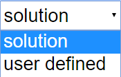
The JavaScript simulation applet offers an interactive environment for users to define resistor networks and potentially input the corresponding matrix equations. While the provided text doesn't detail the applet's interactive solving capabilities, it suggests that it allows users to input variables and possibly directly solve the system. The "User Defined" option hints at the ability to input general matrices and solve them within the applet.

What computational tools are suitable for solving these matrix equations?

Several computational packages are well-suited for solving matrix equations, including Mathematica, Python (with the numpy library, particularly the linalg.solve() function), MatLab, and C/C++ (with appropriate linear algebra libraries). These tools typically provide functions to calculate the inverse of a matrix or directly solve a system of linear equations represented in matrix form.

Why is it important to be able to solve systems of linear equations numerically using computers?

While small systems of linear equations can be solved algebraically, many real-world problems, including complex electrical circuits, mechanical systems, and quantum physics models, involve large and intricate systems of equations. Solving these manually becomes impractical and time-consuming. Numerical methods implemented on computers provide an efficient and accurate way to find solutions for such complex systems.

What are some practical exercises suggested in the provided material?

The material includes two main exercises. The first involves a resistor network with three unknown currents, requiring students to formulate the system of equations using Kirchhoff's Laws, rewrite it in matrix form, solve for the currents using a matrix-solving package, and verify the solutions. The second exercise presents a more complex resistor network, challenging students to repeat the process with a larger system and potentially observe interesting relationships compared to the first exercise under specific conditions.

0.5 1 1 1 1 1 1 1 1 1 1 Rating 0.50 (1 Vote)

Details: Written by Fremont; Parent Category: 05 Electricity and Magnetism; Category: 06 Practical Electricity; Published: 30 May 2018; Created: 30 May 2018; Last Updated: 22 March 2025; Hits: 4215