About

Bungee Oscillation

Activities

 

Translations

Code	Language		Translator	Run

Credits

Leong Tze Kwang; Lawrence Wee Loo Kang; Francisco Esquembre; Felix Garcia Clemente

Overview:

This document provides a briefing on the "Horizontal Spring SVA Graph HTML5 Applet Javascript" resource available on the Open Educational Resources / Open Source Physics @ Singapore website. This resource is an interactive simulation designed to help users visualize and understand the relationship between displacement (x), velocity (v), and acceleration (a) over time (t) for a cart undergoing horizontal oscillations due to a spring. The applet is built using HTML5 and Javascript, making it embeddable and accessible through web browsers.

Main Themes and Important Ideas/Facts:

• Interactive Simulation of Simple Harmonic Motion: The core of this resource is an embeddable HTML5 applet that simulates the motion of a cart attached to a horizontal spring. This allows users to observe the oscillatory behavior directly. The embed code provided is:
• <iframe width="100%" height="100%" src="https://iwant2study.org/lookangejss/02_newtonianmechanics_8oscillations/ejss_model_horizontalspring_sva_graph/_horizontalspring_sva_graph_Simulation.xhtml " frameborder="0"></iframe>
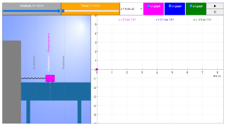
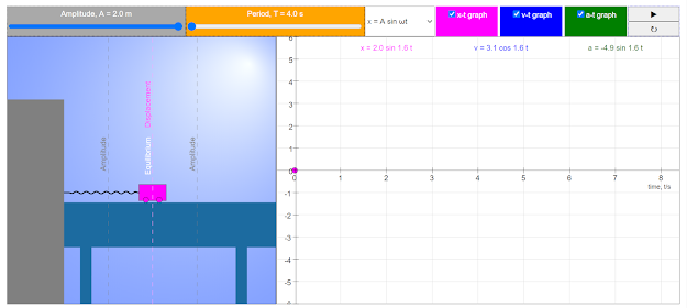
• Visualization of x-t, v-t, and a-t Graphs: A key feature of the simulation is the simultaneous display of graphs showing the cart's displacement, velocity, and acceleration as functions of time. This visual representation helps users connect the physical motion with its graphical representation. The "Initial Setup... displays x-t, v-t, a-t graphs as the cart moves."
• Controllable Variables: The simulation allows users to manipulate key parameters that influence the oscillatory motion. These controllable variables are:
• Amplitude: The maximum displacement of the cart from its equilibrium position.
• Period: The time it takes for one complete oscillation.
• Starting Position: Where the cart begins its motion. These controls enable users to explore how changes in these parameters affect the resulting x-t, v-t, and a-t graphs.
• Open Educational Resource: This resource is part of the Open Educational Resources / Open Source Physics @ Singapore initiative, indicating its commitment to providing free and accessible educational materials. The content is licensed under the "Creative Commons Attribution-Share Alike 4.0 Singapore License," promoting sharing and adaptation.
• Target Audience: Teachers and Students: The resource includes a section "For Teachers" which mentions the initial setup and controllable variables, suggesting it is designed to be used in educational settings. The "Sample Learning Goals" (though the text is empty in the provided excerpt) further reinforce this.
• Credits and Contributors: The applet is credited to Leong Tze Kwang, Lawrence Wee Loo Kang, Francisco Esquembre, and Felix Garcia Clemente, acknowledging the individuals involved in its development.
• Part of a Larger Collection: This specific applet is listed within a broader context of other physics simulations and resources related to oscillations and other topics in Newtonian mechanics. The navigation path shows it under "Oscillations."
• Links to Further Information: A version link (https://weelookang.blogspot.com/2020/07/horizontal-spring-sva-graph-html5.html) is provided, suggesting a blog post or further documentation related to this specific simulation.
• Integration with Other Resources: The page also lists a vast number of other interactive simulations and resources available on the platform, covering a wide range of science and mathematics topics. This indicates a rich ecosystem of open educational materials.

Quotes from the Source:

• "In this simulation, it displays x-t, v-t, a-t graphs as the cart moves." (From "For Teachers" section describing the initial setup)
• "The controllable variables are the Amplitude, Period, and where the cart starts." (From "For Teachers" section outlining user interaction)

Potential Uses:

• Classroom Demonstrations: Teachers can use the interactive simulation to visually demonstrate the concepts of displacement, velocity, and acceleration in simple harmonic motion and how they relate to each other over time.
• Student Exploration: Students can manipulate the amplitude, period, and starting position to observe the resulting changes in the graphs and develop a deeper understanding of the underlying physics.
• Homework and Assignments: The embeddable nature allows teachers to integrate the simulation into online learning platforms or assign it as an interactive exercise.
• Conceptual Understanding: The visual and interactive nature of the applet can aid in building a strong conceptual understanding of oscillatory motion and its graphical representation.

Conclusion:

The "Horizontal Spring SVA Graph HTML5 Applet Javascript" is a valuable open educational resource for teaching and learning about simple harmonic motion. Its interactive nature, clear visualization of kinematic graphs, and controllable parameters make it an effective tool for engaging students and fostering a deeper understanding of the concepts. The fact that it is part of a larger collection of similar resources further enhances its potential for educational use.

 

Horizontal Spring SVA Graph Simulation Study Guide

Overview

This study guide is designed to help you understand the "Horizontal Spring SVA Graph HTML5 Applet Javascript" simulation. This simulation visually represents the motion of a cart attached to a horizontal spring, displaying graphs of its displacement (x), velocity (v), and acceleration (a) as functions of time (t). The simulation allows users to manipulate parameters such as amplitude, period, and starting position to observe the resulting changes in the motion and the corresponding graphs.

Key Concepts

• Oscillation: A repetitive variation, typically in time, of some measure about a central value or between two or more different states. In this simulation, the back-and-forth movement of the cart is an oscillation.
• Simple Harmonic Motion (SHM): A specific type of oscillatory motion where the restoring force is directly proportional to the displacement and acts in the direction opposite to that of displacement. While this simulation shows oscillatory motion, it's important to consider if the conditions strictly adhere to ideal SHM (e.g., no damping).
• Displacement (x): The change in position of the cart from its equilibrium position. In the x-t graph, this is plotted against time.
• Velocity (v): The rate of change of displacement with respect to time. It is the first derivative of the displacement function (v = dx/dt). The v-t graph shows how the cart's velocity changes over time.
• Acceleration (a): The rate of change of velocity with respect to time. It is the second derivative of the displacement function (a = dv/dt = d²x/dt²). The a-t graph illustrates how the cart's acceleration changes over time.
• Amplitude: The maximum displacement of the cart from its equilibrium position. This is a controllable variable in the simulation.
• Period (T): The time taken for one complete oscillation (one full cycle of motion). This is also a controllable variable in the simulation.
• Frequency (f): The number of oscillations per unit time (f = 1/T). Although not directly controllable, it is inversely related to the period.
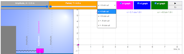
• Phase: The initial position or angle of the oscillating object at time t=0. The "where the cart starts" control in the simulation relates to the initial phase.
• Graphs of Motion: The simulation displays three key graphs:
• Displacement vs. Time (x-t): Shows the position of the cart as it changes over time.
• Velocity vs. Time (v-t): Shows the instantaneous velocity of the cart as it changes over time.
• Acceleration vs. Time (a-t): Shows the instantaneous acceleration of the cart as it changes over time.
• Controllable Variables: The parameters that the user can adjust within the simulation to observe their effects on the motion and graphs (Amplitude, Period, Starting Position).

Quiz

Answer the following questions in 2-3 sentences each.

1. What are the three graphs displayed in the Horizontal Spring SVA Graph simulation, and what does each graph represent?
2. Name the three controllable variables in the simulation that users can adjust. How does changing the amplitude affect the motion of the cart?
3. Explain the relationship between the period and the frequency of oscillation. How would increasing the period affect the displayed graphs?
4. What is displacement in the context of this simulation? How is it represented on the x-t graph?
5. Define velocity and explain its relationship to the displacement graph. What does the slope of the x-t graph represent?
6. Define acceleration and explain its relationship to the velocity graph. What does the slope of the v-t graph represent?
7. How does changing the "where the cart starts" parameter affect the initial conditions of the motion and the starting points of the graphs?
8. What type of motion is being modeled by this simulation? What are the general characteristics of this type of motion?
9. Besides observing the graphs, what other information or insights can be gained by interacting with this simulation?
10. How might this simulation be useful for students learning about oscillations and kinematics?

Quiz Answer Key

1. The three graphs displayed are displacement vs. time (x-t), velocity vs. time (v-t), and acceleration vs. time (a-t). The x-t graph shows the cart's position over time, the v-t graph shows its velocity over time, and the a-t graph shows its acceleration over time.
2. The three controllable variables are Amplitude, Period, and where the cart starts. Changing the amplitude affects the maximum displacement of the cart from its equilibrium position; a larger amplitude means the cart moves further back and forth.
3. Period (T) is the time for one complete oscillation, while frequency (f) is the number of oscillations per unit time. They are inversely related (f = 1/T). Increasing the period would stretch out the oscillations on the time axis of all three graphs, making the cycles longer.
4. Displacement is the change in the cart's position from its resting or equilibrium position. On the x-t graph, the displacement is represented by the vertical distance of the curve from the time axis.
5. Velocity is the rate at which the cart's displacement changes over time. It is the first derivative of displacement. The slope of the x-t graph at any point in time represents the instantaneous velocity of the cart at that moment.
6. Acceleration is the rate at which the cart's velocity changes over time. It is the first derivative of velocity (or the second derivative of displacement). The slope of the v-t graph at any point in time represents the instantaneous acceleration of the cart at that moment.
7. Changing "where the cart starts" alters the initial displacement and consequently the initial velocity of the cart at time t=0. This affects the starting points of the curves on all three graphs, essentially shifting them vertically.
8. This simulation models oscillatory motion, specifically focused on the kinematic aspects (displacement, velocity, acceleration). Oscillatory motion is characterized by a repetitive back-and-forth movement around an equilibrium position.
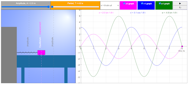
9. By interacting with the simulation, users can visually observe the phase relationships between displacement, velocity, and acceleration in oscillatory motion. They can also see how changing the amplitude and period affects the shape and scale of the respective graphs.
10. This simulation can help students visualize abstract concepts like displacement, velocity, and acceleration in the context of oscillatory motion. It allows them to explore the effects of changing parameters and develop a deeper intuitive understanding of these relationships through graphical representations.

Essay Format Questions

1. Discuss how manipulating the amplitude and period in the Horizontal Spring SVA Graph simulation affects the displacement, velocity, and acceleration graphs. Analyze the relationships between these changes and the underlying physics of oscillatory motion.
2. Explain the phase relationships between displacement, velocity, and acceleration in the context of the Horizontal Spring SVA Graph simulation. How are these relationships visually represented in the x-t, v-t, and a-t graphs?
3. Consider the "Horizontal Spring SVA Graph HTML5 Applet Javascript" as a tool for teaching and learning about kinematics and oscillations. What are the strengths and limitations of using such a simulation in an educational setting?
4. Relate the motion depicted in the Horizontal Spring SVA Graph simulation to real-world examples of oscillatory motion. Discuss the similarities and potential differences between the idealized simulation and actual physical systems.
5. Describe how you would use the Horizontal Spring SVA Graph simulation to demonstrate and explain the concepts of simple harmonic motion to a student. What specific observations and manipulations would you guide them through?

Glossary of Key Terms

• Amplitude: The maximum extent of a vibration or oscillation, measured from the position of equilibrium.
• Acceleration: The rate at which the velocity of an object changes with respect to time, in both speed and direction.
• Displacement: The change in position of an object from its equilibrium or starting point, usually a vector quantity having both magnitude and direction. In this context, it's the horizontal distance from the resting position.
• Frequency: The number of cycles or oscillations per unit time, usually measured in Hertz (Hz), where 1 Hz = 1 cycle per second.
• Oscillation: A repetitive variation, typically in time, of some measure about a central value or between two or more different states.
• Period: The time taken for one complete cycle of an oscillation or vibration. It is the reciprocal of the frequency (T = 1/f).
• Phase: The fraction of a cycle that has elapsed relative to some arbitrary starting point, often expressed as an angle in radians or degrees. It indicates the initial state of an oscillation.
• Simulation: A computer-based model that mimics the behavior of a real-world system, allowing users to interact with and observe the effects of different parameters.
• Velocity: The rate of change of an object's position with respect to time and a frame of reference, a vector quantity with both magnitude (speed) and direction.

Sample Learning Goals

[text]

For Teachers

 

Research

[text]

Video

[text]

 Version:

1. https://weelookang.blogspot.com/2020/07/horizontal-spring-sva-graph-html5.html 

Other Resources

[text]