PICUP Solving Systems of Linear Equations Resistor Networks JavaScript Simulation Applet HTML5

Breadcrumbs

About

1instructorguide

These exercises are designed to get students started on using computers to solve systems of linear equations. Students should have some experience in an appropriate computational package before attempting this. Mathematica is a very good choice of tools for this exercise, closely followed by Python/numpy and MatLab. C/C++ also works, with appropriate libraries. The systems of equations we’ll be using come from resistor networks typical of a second-semester physics course, but the same techniques can be used for any system of linear equations regardless of their source.

Being able to solve systems of equations is an important computational skill, with applications in everything from mechanical engineering to quantum physics. For small systems of equations it is fairly simple to solve the systems algebraically, but for large complex systems it’s important to be able to solve them numerically using computers.

2theory

We first express the system of equations as a single matrix equation,

\begin{matrix} (1) & M x = b \end{matrix}

Since there are as many equations (rows in $M$ ) as there are variables (columns in $M$ ), $M$ will be a square matrix. If there is a solution to this set of equations, then there will exist another matrix $M^{- 1}$ such that $M^{- 1} M = I$ , where $I$ is the identity matrix. In that case,

\begin{matrix} (2) & M^{- 1} M x = M^{- 1} b \end{matrix}

\begin{matrix} (3) & I x = x = M^{- 1} b \end{matrix}

There are algorithmic methods for finding $M^{- 1}$ (and thus $x$ ; in our case we’ll be using standard libraries to calculate this matrix and the corresponding solution. One standard method is to have the computer calculate $M^{- 1}$ directly using an “invert()” function, and then multiply that inverse matrix by $b$ to obtain $x$ .

Most computational packages that have the ability to calculate $M^{- 1}$ also have an additional function, often called “solve()”, that takes care of the multiplication as well, and gives the user $x$ directly.

For more information about how these functions work, see Numerical Recipes in C by Flannery, Teukolsky, Press, and Vetterling, or similar text.

3exercises

Exercise 1: Introductory Problem

Consider the network of resistors and batteries shown in the first figure below.

There are three unknowns in that circuit, $I_{1}$ , $I_{2}$ , and $I_{3}$ . We can solve for these unknowns by building a system of equations using Kirchhoff’s Laws:

The sum of voltages around any loop is zero.
The sum of currents at any junction is zero.

Applying the voltage law to the left-hand loop, we get

\begin{matrix} (4) & V_{1} - I_{1} R_{1} - I_{3} R_{3} = 0 \end{matrix}

From the right-hand loop, we get

\begin{matrix} (5) & V_{2} + I_{2} R_{2} - I_{3} R_{3} = 0 \end{matrix}

We need one more equation, for which we can use the junction at top center and the current law:

\begin{matrix} (6) & I_{1} - I_{2} - I_{3} = 0 \end{matrix}

We now have the requisite three independent equations, which we can solve using methods learned in high-school algebra.

There’s another way of solving this, using matrix methods. First, rewrite the equations just a bit.

\begin{aligned} (7) & R_{1} I_{1} + 0 I_{3} + R_{3} I_{3} & = & V_{1} \\ (8) & 0 I_{1} - R_{2} I_{2} + R_{3} I_{3} & = & V_{2} \\ (9) & I_{1} - I_{2} - I_{3} & = & 0 \end{aligned}

And now we can see that this can be written as a matrix equation!

\begin{matrix} (10) & [\begin{matrix} R_{1} & 0 & R_{3} \\ 0 & - R_{2} & R_{3} \\ 1 & - 1 & - 1 \end{matrix}] [\begin{matrix} I_{1} \\ I_{2} \\ I_{3} \end{matrix}] = [\begin{matrix} V_{1} \\ V_{2} \\ 0 \end{matrix}] \end{matrix}

This matrix equation,

\begin{matrix} (11) & M x = b \end{matrix}

has solution

\begin{matrix} (12) & x = M^{- 1} b \end{matrix}

where $M^{- 1}$ is the inverse of $M$ . Most computational packages have built-in capability for inverting matrices.

ASSIGNMENT

By carrying out the matrix multiplication explicitly, show that the matrix equation above reduces to the system of equations from which it is derived.
Use a matrix-solving package to find the currents.
Check your answers by substituting the currents into the equations and verifying that they are solutions.

Exercise 2: More complicated problem

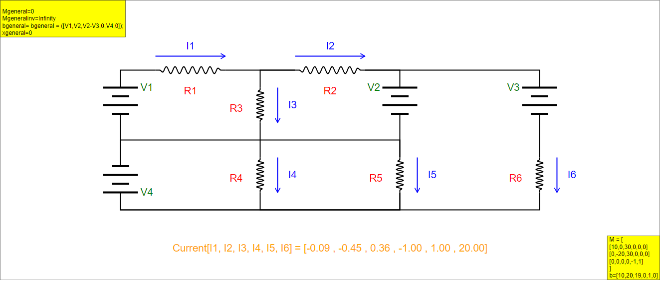
The resistor network below is perhaps a bit more challenging.

ASSIGNMENT

Write a system of equations that can be used to solve for the currents in the circuit above.
Re-write the system of equations from part 1 of this assignment as a matrix equation.
Use a matrix-solving package to find the currents.
Check your answers: do the values of currents you found solve the equations with which you started?
You may notice something interesting if you compare your solution here to your solution for exercise 1. (Assuming the same values of $R$ and $V$ were used in both exercises.) Explain why this happened.

Unless your instructor provides you with other values, assume each voltage source and each resistor has a value $10 \times$ its identifying number. (i.e. $V_{2} = 20$ V, $R_{3} = 30 Ω$ .)

5solutions

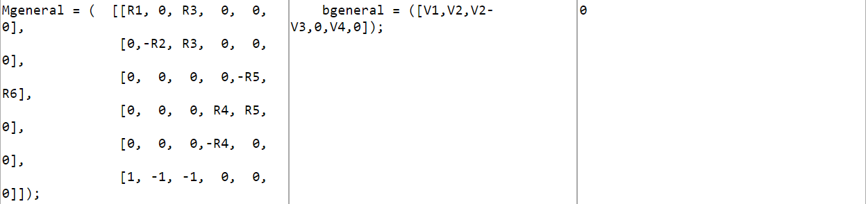
The set of equations from the assigned problem will vary, here is one possible set.

\begin{matrix} (13) & V_{1} - R_{1} I_{1} - R_{3} I_{3} = 0 \end{matrix}

\begin{matrix} (14) & - R_{2} I_{2} - V_{2} + R_{3} I_{3} = 0 \end{matrix}

\begin{matrix} (15) & V_{2} - V_{3} - R_{6} I_{6} + R_{5} I_{5} = 0 \end{matrix}

\begin{matrix} (16) & R_{4} I_{4} - R_{5} I_{5} = 0 \end{matrix}

\begin{matrix} (17) & - V_{4} - R_{4} I_{4} = 0 \end{matrix}

\begin{matrix} (18) & I_{1} - I_{2} - I_{3} = 0 \end{matrix}

This set of equations can be converted to the following matrix equation:

\begin{matrix} (19) & [\begin{matrix} R_{1} & 0 & R_{3} & 0 & 0 & 0 \\ 0 & - R_{2} & R_{3} & 0 & 0 & 0 \\ 0 & 0 & 0 & 0 & - R_{5} & R_{6} \\ 0 & 0 & 0 & R_{4} & R_{5} & 0 \\ 0 & 0 & 0 & - R_{4} & 0 & 0 \\ 1 & - 1 & - 1 & 0 & 0 & 0 \end{matrix}] [\begin{matrix} I_{1} \\ I_{2} \\ I_{3} \\ I_{4} \\ I_{5} \\ I_{6} \end{matrix}] = [\begin{matrix} V_{1} \\ V_{2} \\ V_{2} - V_{3} \\ 0 \\ V_{4} \\ 0 \end{matrix}] \end{matrix}

The answers are

\begin{matrix} (20) & I_{1} = - 0.091 \end{matrix}

\begin{matrix} (21) & I_{2} = - 0.455 \end{matrix}

\begin{matrix} (22) & I_{3} = 0.364 \end{matrix}

\begin{matrix} (23) & I_{4} = - 1 \end{matrix}

\begin{matrix} (24) & I_{5} = 0.8 \end{matrix}

\begin{matrix} (25) & I_{6} = 0.5 \end{matrix}

It should be noted that for the circuit in the second figure, currents $I_{1}$ through $I_{3}$ are the same as for the first figure, and it may be interesting to discuss with students why that should be the case.

solutionpy

'''

solution.py

Eric Ayars

June 2016

A solution of the 5-loop circuit exercise.

'''

import numpy as np

# Start by getting the values of R and V

R1 = float(input("R1 = "))

R2 = float(input("R2 = "))

R3 = float(input("R3 = "))

R4 = float(input("R4 = "))

R5 = float(input("R5 = "))

R6 = float(input("R6 = "))

V1 = float(input("V1 = "))

V2 = float(input("V2 = "))

V3 = float(input("V3 = "))

V4 = float(input("V4 = "))

# Use these values to build the matrix M. Note that this matrix

# will vary depending on the equation set selected to solve the

# problem: here I use the equations from the solution on the

# PICUP webpage.

M = np.array([ [R1, 0, R3, 0, 0, 0],

[0,-R2, R3, 0, 0, 0],

[0, 0, 0, 0,-R5, R6],

[0, 0, 0, R4, R5, 0],

[0, 0, 0,-R4, 0, 0],

[1, -1, -1, 0, 0, 0] ])

# here is the right-hand-side b:

b = np.array([V1,V2,V2-V3,0,V4,0])

# And this is all it takes to get a solution:

x = np.linalg.solve(M,b)

# show the result.

print(x)

Translations

Code	Language		Translator	Run

Credits

Fremont Teng; Loo Kang Wee

Source: Excerpts from "PICUP Solving Systems of Linear Equations Resistor Networks JavaScript Simulation Applet HTML5 - Open Educational Resources / Open Source Physics @ Singapore"

Date: Generated based on provided source excerpts.

Overview:

This document provides a briefing on the PICUP (Partnership for Integration of Computation into Undergraduate Physics) resource focused on solving systems of linear equations using resistor networks as a practical application. The resource includes a JavaScript simulation applet and accompanying instructor guide with exercises designed to introduce students to computational methods for solving linear systems, a fundamental skill with broad applications in physics and engineering.

Main Themes and Important Ideas/Facts:

Using Computational Tools for Solving Linear Equations: The core theme of this resource is to introduce students to the power of using computers to solve systems of linear equations. While algebraic methods are suitable for small systems, the resource emphasizes the necessity of numerical methods for larger, more complex systems. The instructor guide explicitly recommends computational packages like Mathematica, Python/numpy, and MatLab, noting that C/C++ can also be used with appropriate libraries.

Quote: "For small systems of equations it is fairly simple to solve the systems algebraically, but for large complex systems it’s important to be able to solve them numerically using computers."

Application to Resistor Networks: The resource uses resistor networks, a common topic in second-semester physics courses, as the source of the linear equations. This provides a tangible and relevant context for students to understand the application of these mathematical techniques. However, the resource clearly states that the methods learned are applicable to "any system of linear equations regardless of their source."

Quote: "The systems of equations we’ll be using come from resistor networks typical of a second-semester physics course, but the same techniques can be used for any system of linear equations regardless of their source."

Matrix Representation of Linear Equations: The theoretical basis for solving these systems computationally involves expressing them as a matrix equation in the form M x = b, where M is the coefficient matrix, x is the vector of unknowns (e.g., currents), and b is the constant vector (e.g., voltages).

Quote: "We first express the system of equations as a single matrix equation, M x = b (1)"

Solving using Matrix Inversion: The document explains the concept of the inverse of a matrix (M⁻¹) and how it can be used to solve the system (x = M⁻¹ b). It notes that computational packages often provide functions to directly calculate the inverse or, more efficiently, a "solve()" function that directly yields the solution vector x.

Quote: "If there is a solution to this set of equations, then there will exist another matrix M − 1 such that M − 1 M = I , where I is the identity matrix. In that case, I x = x = M − 1 b (3)"
Quote: "Most computational packages that have the ability to calculate M − 1 also have an additional function, often called “solve()”, that takes care of the multiplication as well, and gives the user x directly."

Exercises Based on Kirchhoff's Laws: The resource includes two exercises involving resistor networks. Exercise 1 is an introductory problem with three unknowns, requiring students to apply Kirchhoff's Voltage Law (sum of voltages around a loop is zero) and Kirchhoff's Current Law (sum of currents at a junction is zero) to derive a system of three linear equations. This system is then rewritten in matrix form.

Quote (Kirchhoff's Laws): "1. The sum of voltages around any loop is zero. 2. The sum of currents at any junction is zero."
Quote (Exercise 1 Matrix Equation):
[ R1 0 R3 ] [ I1 ] [ V1 ]
[ 0 -R2 R3 ] [ I2 ] = [ V2 ]
[ 1 -1 -1 ] [ I3 ] [ 0 ]

A More Complex Problem: Exercise 2 presents a more complex resistor network, requiring students to develop a larger system of equations (potentially six unknowns as suggested by the solution) and represent it as a matrix equation. This exercise reinforces the process and highlights the efficiency of computational methods for more involved circuits.
Importance of Verification: Both exercises include the crucial step of verifying the obtained solutions by substituting the calculated currents back into the original equations. This emphasizes the need for accuracy and understanding of the solution.

Quote (Assignment 3 in Exercise 1): "Check your answers by substituting the currents into the equations and verifying that they are solutions."

JavaScript Simulation Applet: The resource includes an embedded JavaScript simulation applet, suggesting an interactive component where students can potentially manipulate circuit parameters and observe the resulting currents, although the specific functionalities of the applet are not detailed in the provided excerpts beyond the embedding instructions and combo box functions for "Solution" and "user defined" matrix input.
Instructor Guidance and Open Educational Resource: The resource is presented as an Open Educational Resource (OER) from Open Source Physics @ Singapore, indicating it is freely available for educational use. The "instructorguide" section suggests it is designed to support educators in using this material with their students.
Python Solution Example: A Python script using the numpy library is provided as a solution to the more complex (5-loop) circuit. This demonstrates the practical implementation of solving such systems using computational tools. The script takes resistor and voltage values as input and uses np.linalg.solve() to find the currents.
Connections to Broader Applications: The introduction explicitly states the broad applicability of solving linear equations, ranging from "mechanical engineering to quantum physics," underscoring the importance of this skill beyond the context of electrical circuits.

Quote: "Being able to solve systems of equations is an important computational skill, with applications in everything from mechanical engineering to quantum physics."

Key Assignments for Students:

Expressing circuit problems using Kirchhoff's Laws to form systems of linear equations.
Representing these systems of equations in matrix form (M x = b).
Using computational tools (matrix-solving packages) to find the unknown currents.
Verifying the obtained solutions.
Analyzing and explaining observations when comparing solutions from different (but related) circuit configurations.

In Conclusion:

This PICUP resource provides a valuable pedagogical tool for introducing students to the computational solution of linear equations within the familiar context of resistor networks. By combining theoretical explanations, practical exercises, a JavaScript simulation applet, and example code, it aims to equip students with a fundamental computational skill applicable across various scientific and engineering disciplines. The emphasis on matrix representation and the use of computational packages reflects the modern approach to solving complex problems in physics and related fields.

Solving Systems of Linear Equations in Resistor Networks

Study Guide

This study guide is designed to help you review the concepts and techniques presented in the PICUP resource for solving systems of linear equations, specifically within the context of resistor networks.

I. Key Concepts

Systems of Linear Equations: Understand what constitutes a system of linear equations, where multiple equations contain multiple variables to be solved simultaneously.
Matrix Representation of Linear Equations: Be able to represent a system of linear equations in the form of a matrix equation: (Mx = b), where (M) is the coefficient matrix, (x) is the column vector of unknowns, and (b) is the column vector of constants.
Kirchhoff's Laws: Understand and be able to apply Kirchhoff's Voltage Law (the sum of voltages around any closed loop in a circuit is zero) and Kirchhoff's Current Law (the sum of currents entering any junction in a circuit is zero) to set up systems of equations for resistor networks.
Matrix Inverse: Understand the concept of a matrix inverse ((M^{-1})) and its property that (M^{-1}M = I), where (I) is the identity matrix.
Solving Matrix Equations using Inverse: Understand how the inverse of the coefficient matrix can be used to solve for the unknown vector (x) in a matrix equation: (x = M^{-1}b).
Computational Packages for Solving Linear Equations: Recognize the utility of computational tools (like Mathematica, Python/NumPy, and MatLab) in solving large systems of linear equations using functions such as invert() and solve().
Identity Matrix: Understand the properties of an identity matrix, particularly its role in matrix multiplication ((Ix = x)).

II. Practical Applications

Resistor Networks: Understand how systems of linear equations arise when analyzing resistor networks using Kirchhoff's Laws to determine unknown currents.
General Applicability: Recognize that the techniques for solving systems of linear equations using matrices are not limited to resistor networks and can be applied to various problems in fields like mechanical engineering and quantum physics.

III. Exercises Review

Exercise 1: Introductory Problem:Review how the system of three linear equations for the three unknown currents ((I_1), (I_2), (I_3)) is derived from Kirchhoff's Laws applied to the given circuit.
Understand the process of rewriting these equations in matrix form ((Mx = b)).
Reflect on the assignment tasks: explicitly performing the matrix multiplication to recover the original equations, using a matrix-solving package to find the currents, and verifying the solutions.
Exercise 2: More Complicated Problem:Analyze the more complex resistor network and consider how to apply Kirchhoff's Laws to generate a larger system of linear equations to solve for the unknown currents.
Understand how to represent this larger system as a matrix equation.
Think about the significance of comparing the solutions of this exercise to the first one when assuming the same component values. What does it imply about the behavior of certain parts of the circuit?

IV. Computational Tools

Understand that computational packages provide efficient ways to find the inverse of a matrix and solve systems of linear equations numerically, especially for larger and more complex systems where algebraic solutions become impractical.

Quiz

Answer the following questions in 2-3 sentences each.

What are the two fundamental laws governing electrical circuits that are used to set up systems of linear equations for resistor networks?
Explain how a system of linear equations representing a resistor network can be written in the form of a matrix equation (Mx = b). What do (M), (x), and (b) represent in this context?
What is the significance of the inverse of the coefficient matrix ((M^{-1})) in solving a matrix equation of the form (Mx = b)?
For what types of systems of linear equations is it particularly important to be able to solve them numerically using computers rather than algebraically?
Describe one standard method that computational packages use to solve a matrix equation (Mx = b) for the unknown vector (x).
In the context of the first exercise, how were the three linear equations derived from the resistor network? Briefly mention the loops and junction considered.
What was the assignment in the first exercise that required explicitly performing matrix multiplication? What was the purpose of this task?
In the second, more complicated problem, what is the first step in setting up the solution to find the unknown currents in the circuit?
According to the provided solution for the second exercise, what interesting observation can be made when comparing the currents (I_1) through (I_3) with the solution of the first exercise (assuming identical component values)?
What general computational skill is emphasized by the exercises in the PICUP resource, and in what diverse fields can this skill be applied?

Quiz Answer Key

The two fundamental laws are Kirchhoff's Voltage Law (KVL), which states that the sum of voltages around any closed loop is zero, and Kirchhoff's Current Law (KCL), which states that the sum of currents at any junction is zero. These laws provide the relationships needed to form the system of equations.
In the matrix equation (Mx = b), (M) is the coefficient matrix containing the resistances and coefficients of the currents from the equations, (x) is the column vector representing the unknown currents ((I_1, I_2, I_3), etc.), and (b) is the column vector containing the voltage sources (constants) from the equations.
The inverse of the coefficient matrix, (M^{-1}), allows us to isolate the unknown vector (x) by multiplying both sides of the matrix equation by (M^{-1}). Since (M^{-1}M) equals the identity matrix (I), and (Ix = x), the solution becomes (x = M^{-1}b).
It is particularly important to solve large and complex systems of linear equations numerically using computers because algebraic methods become very tedious, time-consuming, and prone to errors with an increasing number of variables and equations.
One standard method involves the computer calculating the inverse of the coefficient matrix (M) using an "invert()" function. Then, the solution vector (x) is obtained by multiplying this inverse matrix (M^{-1}) by the constant vector (b).
The three linear equations in the first exercise were derived by applying Kirchhoff's Voltage Law to the left-hand loop ((V_1 - I_1R_1 - I_3R_3 = 0)), the right-hand loop ((V_2 + I_2R_2 - I_3R_3 = 0)), and Kirchhoff's Current Law to the junction at the top center ((I_1 - I_2 - I_3 = 0)).
The assignment was to multiply the coefficient matrix and the column vector of currents explicitly and show that the result is equal to the column vector of voltages and zero. The purpose was to demonstrate the equivalence between the matrix equation and the original system of linear equations.
The first step in setting up the solution for the more complicated problem is to apply Kirchhoff's Voltage Law to each independent loop in the circuit and Kirchhoff's Current Law to sufficient junctions to create a system of independent linear equations that includes all the unknown currents.
Assuming the same values for resistors ((R)) and voltage sources ((V)) were used in both exercises, the currents (I_1) through (I_3) are the same for both circuits. This suggests that the added components in the second circuit do not affect the current distribution in the initial part of the network.
The exercises emphasize the important computational skill of being able to solve systems of linear equations. This skill has broad applications in diverse fields ranging from mechanical engineering and electrical engineering to quantum physics and many other areas of science and technology.

Essay Format Questions

Discuss the role of Kirchhoff's Laws in transforming a physical resistor network into a mathematical problem solvable by linear algebra. Explain how these laws lead to the formation of a system of linear equations.
Explain the theoretical basis for using matrix methods, specifically the matrix inverse, to solve systems of linear equations. Why is this approach particularly powerful for complex systems?
Compare and contrast the process of solving a system of linear equations algebraically versus using computational packages. What are the advantages and disadvantages of each method, especially in the context of analyzing electrical circuits?
The PICUP resource highlights the use of computational packages like Mathematica, Python/NumPy, and MatLab. Discuss the general capabilities these tools offer for solving mathematical problems in physics and engineering beyond just linear equations.
Analyze the two resistor network problems presented in the resource. How does the complexity of the circuit impact the system of linear equations needed for its solution, and what insights can be gained by comparing the results of the two exercises?

Glossary of Key Terms

System of Linear Equations: A set of two or more linear equations containing two or more variables for which a common solution is sought.
Matrix: A rectangular array of numbers, symbols, or expressions, arranged in rows and columns.
Vector: A quantity having direction as well as magnitude, often represented as a column or row of numbers (a matrix with one column or one row). In this context, it refers to the unknowns or the constants in the system of equations.
Coefficient Matrix (M): A matrix whose elements are the coefficients of the variables in a system of linear equations.
Unknown Vector (x): A column vector containing the variables for which the system of linear equations is being solved.
Constant Vector (b): A column vector containing the constant terms on the right-hand side of a system of linear equations.
Matrix Equation (Mx = b): A compact representation of a system of linear equations using matrices and vectors.
Matrix Inverse (M⁻¹): A matrix that, when multiplied by the original square matrix (M), yields the identity matrix (I).
Identity Matrix (I): A square matrix with 1s on the main diagonal and 0s elsewhere. It has the property that when multiplied by any other matrix, it leaves the other matrix unchanged.
Kirchhoff's Voltage Law (KVL): The principle that the algebraic sum of the voltages around any closed loop in an electrical circuit must be zero.
Kirchhoff's Current Law (KCL): The principle that the algebraic sum of currents entering and leaving any junction (node) in an electrical circuit must be zero.
Computational Package: Software equipped with tools and functions for performing numerical and symbolic computations, such as solving systems of equations, inverting matrices, and more (e.g., Mathematica, Python with NumPy/SciPy, MatLab).
invert() function: A function in computational packages that calculates the inverse of a given square matrix.
solve() function: A function in computational packages that directly finds the solution vector for a system of linear equations given the coefficient matrix and the constant vector, often more efficiently than explicitly calculating the inverse.
Resistor Network: An electrical circuit containing interconnected resistors and possibly voltage or current sources.
Current (I): The rate of flow of electric charge, typically measured in amperes (A).
Voltage (V): The electric potential difference between two points, typically measured in volts (V).
Resistance (R): A measure of the opposition to the flow of electric current, typically measured in ohms (Ω).

Sample Learning Goals

[text]

For Teachers

Solving Systems of Linear Equations Resistor Networks JavaScript Simulation Applet HTML5

Instructions

Combo Box and Functions

Toggling through the combo box will give you their respective functions.

Selecting Solution will give you their respective input fields for

the variables as shown in the diagram above.

Selecting user defined allow you to customise the matrix

of Mgeneral and bgeneral to solve any equation.

Note that putting an invalid matrix/solution will catch you an error message.

Toggling Full Screen

Click anywhere inside the panel to toggle full screen.

Reset Button

Resets the simulation.

Research

[text]

Video

[text]

Version:

Other Resources

[text]

Frequently Asked Questions: Solving Linear Equations with Resistor Networks

What is the purpose of the provided JavaScript simulation applet? The applet is designed to help students learn how to use computational tools to solve systems of linear equations. It uses the context of resistor networks, a common topic in second-semester physics, to illustrate these mathematical techniques. The underlying principle, however, applies to any system of linear equations, regardless of its origin, making it a versatile educational resource.
Why is solving systems of linear equations considered an important skill? Solving systems of linear equations is a fundamental computational skill with broad applications across various scientific and engineering disciplines. These applications range from mechanical engineering and electrical engineering (like analyzing circuits) to more advanced fields like quantum physics. The ability to solve these systems numerically, especially for large and complex problems, is essential in modern scientific research and development.
How are systems of linear equations related to resistor networks? The behavior of resistor networks, particularly the currents flowing through different resistors, can be described by a system of linear equations derived from Kirchhoff's circuit laws (Kirchhoff's voltage law and Kirchhoff's current law). By applying these laws to the loops and junctions within a resistor network, a set of linear equations can be formulated where the unknown variables are the currents in the circuit.
How can a system of linear equations be represented using matrices? A system of linear equations can be concisely expressed in the form of a matrix equation, typically written as M x = b. Here, M is the coefficient matrix containing the coefficients of the unknown variables from each equation, x is the column vector representing the unknown variables (e.g., currents in a circuit), and b is the column vector containing the constant terms (e.g., voltage sources).
What is the significance of the inverse of a matrix (M⁻¹)? If the coefficient matrix M is a square matrix and a solution to the system of linear equations exists, then M will have an inverse, denoted as M⁻¹. Multiplying both sides of the matrix equation M x = b by M⁻¹ yields x = M⁻¹ b. This means that the solution vector x can be found by multiplying the inverse of the coefficient matrix by the constant vector.
How do computational packages help in solving these matrix equations? Computational packages like Mathematica, Python (with numpy), and MatLab provide built-in functions to perform matrix operations, including finding the inverse of a matrix and solving systems of linear equations. These packages often have functions like "invert()" to calculate the inverse matrix directly and "solve()" which can directly compute the solution vector x by handling the matrix inversion and multiplication steps efficiently.
What are Kirchhoff's Laws and how are they used to formulate equations for resistor networks? Kirchhoff's Laws are fundamental principles in circuit analysis. Kirchhoff's Voltage Law (KVL) states that the sum of the voltages around any closed loop in a circuit must be zero. Kirchhoff's Current Law (KCL) states that the sum of the currents entering any junction (node) in a circuit must be zero. By applying KVL to different loops and KCL to different junctions in a resistor network, we can generate a set of independent linear equations that describe the relationships between the voltages, resistances, and currents in the circuit.
What is the educational value of working through the provided exercises with resistor networks? The exercises provide a practical context for understanding and applying the mathematical techniques of solving systems of linear equations. By starting with a relatively simple resistor network and progressing to a more complex one, students can see how real-world problems can be translated into mathematical models. Furthermore, by using computational tools to solve these systems and then verifying the solutions, students develop both their problem-solving and computational skills, as well as gain a deeper understanding of the underlying physical principles of electricity.

1 1 1 1 1 1 1 1 1 1 Rating 0.00 (0 Votes)

Details: Written by Fremont; Parent Category: 05 Electricity and Magnetism; Category: 06 Practical Electricity; Published: 30 May 2018; Created: 30 May 2018; Last Updated: 22 March 2025; Hits: 4469