About

Subject Area	Mechanics
Levels	First Year and Beyond the First Year
Available Implementations	C/C++, Fortran, IPython/Jupyter Notebook, Mathematica, Octave*/MATLAB, Python, Spreadsheet and Easy JavaScript Simulation
Learning Objectives	Students who complete this set of exercises will be able to build a computational model of a simple rigid pendulum using the Euler-Cromer algorithm (Exercise 1); to produce graphs of the angular displacement and angular velocity of the pendulum as a function of time from the results of their computational model (Exercises 1-5); to assess the accuracy of the computational results of their model (Exercises 1); to identify the limitations of the small angle approximation for the plane pendulum (Exercises 2) to produce phase space plots for various system parameters (Exercises 3); and to produce chaotic phase space trajectories by varying model parameters (Exercise 4 and 5);

For this Exercise Set, I have chosen a rigid pendulum, rather than a mass suspended from a massless string, so that angular displacements of magnitude greater than π/2$\pi /2$ can be studied, without concern for the mass remaining at the same location relative to the support. The stable Euler Cromer method is employed; however, the instructor could have the students start out with an “Exercise 0” that asks students to use the simple Euler method to model the pendulum. The Euler algorithm is unstable for oscillatory systems (total energy grows every time step), and this exercise could provide a valuable lesson in the control of artificial behavior in computational models, and the importance of using stable algorithms. Even if this “Exercise 0” were implemented, it might be best if students have already had experience modeling and studying the dynamics of a simpler oscillatory system, such as the Simple Hanging Harmonic Oscillator in the PICUP collection, before encountering the Rigid Pendulum exercise set.

Exercise 1 asks the students to build the computational model of the hanging spring-mass system. Depending on instructor preference, a working version of the computational model could be directly provided to the student; or the student could be required to modify, or add to, a nearly completed computational model; or the student required to build the model from scratch; or really anything in between these scenarios. Another possibility for producing a working model, time permitting, is to build it, or parts of it, together with the students in class. To carry out the subsequent exercises the student must have the working program, and also access to either a plotting program, or a programming environment with built-in graphics capabilities.

The student should be made aware of the analytic solution of the (undamped and unforced) rigid pendulum accessible via the small angle approximation. The second exercise in this set has the students compare this small angle solution to their computational one. Also, the concept of phase space is presented in the exercises as simply another way of plotting and observing the system dynamics. Adding the damping and driving terms in exercises 4 and 5, and guiding the students to explore the behavior for different parameter values, serves as a basic introduction to nonlinear dynamics.

This computational approach to the rigid pendulum has the educational advantage of allowing introductory students to study the dynamics of a nonlinear, chaotic system with relative computational ease.

Consider a uniform rigid bar of mass m$m$ and length L$L$ that has been fastened to a stationary support at point P, as shown in the figure below. Assume that the bar is constrained to rotate in a 2D vertical plane when it is displaced from its vertical equilibrium position and released.

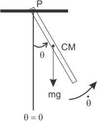
The figure shows the pendulum at an instant in time in which it is rotating in a counterclockwise direction with angular speed θ˙$\dot{\theta }$, and has an angular displacement of θ$\theta$ with respect to its equilibrium (θ=0)$\theta =0)$ position. If we neglect forces that produce any damping or driving torques, then the bar’s weight is the only force exerted on the bar that produces a torque about point P. In the figure the weight mg$mg$ of the bar is represented by the force vector drawn at the position of the bar’s center of mass CM. We shall use a sign convention such that any torque that tries to produce an angular acceleration in the counterclockwise direction contributes a positive amount to the total torque acting on the bar, and any torque that tries to accelerate the bar in the clockwise direction is a negative contribution. With this sign convention the torque exerted on the rigid bar by its weight is

The rotational analog to Newton’s 2nd Law of motion is

where I$I$ is the moment of inertia of the bar about the point P, and θ¨$\ddot{\theta }$ is the angular acceleration. If we consider all of the bar’s mass to be concentrated at the position of its center of mass, then

Inserting Equations (1$\text{1}$) and (3$\text{3}$) into (2$\text{2}$), and a little rearranging produces

for the angular acceleration.

If we include the influence of a damping torque, that acts to oppose the rotational motion of the bar, and a sinusoidal driving torque, then

With the bar rotating in a counterclockwise direction, the damping torque tries to accelerate the bar in the clockwise direction. Thus, like the torque due to gravity, the sign of the damping torque is negative. For the damping torque we use τdamping=−bθ˙${\tau }_{damping}=-b\dot{\theta }$, where b$b$ is a constant, and has units of kg⋅m2/s$\text{kg}\cdot {\text{m}}^2/s$. The constant b$b$can be thought of as an effective “damping strength” that characterizes the damping effects due to air resistance as the bar rotates through the atmospheric fluid, and any friction between the bar and the supporting mechanism at point P. For the driving torque we use τdriving=τdcosωt${\tau }_{driving}={\tau }_d\cos \omega t$, where τd${\tau }_d$ is the amplitude and ω$\omega$ is the driving frequency in rad/s. Thus, Equation (5$\text{5}$) becomes

Solving for the angular acceleration we arrive at

for the rigid damped driven pendulum.

See the pseudocode for the implementation of the Euler-Cromer algorithm for solving Equation 7$\text{7}$.

Exercise 1: Euler-Cromer Model of the Rigid Pendulum

Build a computational model of a plane undamped, unforced rigid pendulum using the Euler-Cromer method. Assume your pendulum consists of a rigid metallic rod, one meter in length, with a mass of 1kg. Also assume that one end of the rod is fixed to an immovable support, and that the rod is free to rotate without bound in a plane. For initial conditions, assume the rod is displaced at some angle, greater than 90∘${90}^{\circ }$, relative to its vertical minimum potential energy configuration, and released from rest. This physical situation has no exact analytical solution with which you will be able to compare the results of your computational model, so you must carefully determine a value of Δt$\mathrm{\Delta }t$ that produces an accurate approximation without the benefit of making a comparison. Describe in detail the procedure you used in arriving at an acceptably small value of Δt$\mathrm{\Delta }t$, show plots of the angular displacement and angular velocity as functions of time, and comment on the pendulum’s dynamic behavior. Is the behavior of your computational model what you expect for a real pendulum?

Exercise 2: Comparison with Analytical Small Angle Approximation Solution

Once you have determined a value of Δt$\mathrm{\Delta }t$ that produces an acceptably accurate computational solution, compare the computational results (angular displacement as a function of time) with the analytically determined function for the angular displacement

for the rigid pendulum, resulting from the small angle approximation. Comment in detail on your observations.

Exercise 3: Phase Space

A very useful plot for analyzing periodic systems is known as a phase space plot, and is simply a graph of velocity vs. position. The resulting curve is known as a phase space trajectory. In the case of the plane rigid pendulum, the phase space trajectory is found by graphing angular velocity vs. angular displacement. Produce a phase space plot for the plane pendulum using the parameters and initial conditions you used (including an accurate value for Δt$\mathrm{\Delta }t$ !) in Exercise 1. Comment in detail on the resulting phase space trajectory.

Exercise 4: Damped Rigid Pendulum

Now, add a damping term to your pendulum model. Explore, and produce graphs of (time dependent behavior as well as phase space), the behavior of the model by systematically varying the damping strength b$b$ . Use the same values for the physical parameters and initial conditions as before. Describe the effect of increasing the damping strength, while keeping the other parameters the same. Can you damp the pendulum to such an extent that it doesn’t actually oscillate?

Exercise 5: Damped, Driven Rigid Pendulum

Next add a driving torque to your pendulum model. Once you’re sure that your model is accurately computing the damped, driven pendulum’s dynamics, systemically explore the behavior of the model by varying the driving torque amplitude τd${\tau }_d$ . Use the same physical parameters and initial conditions as before, including values of b$b$ = 0.2 and ω$\omega$ = 3 rad/s for the damping strength and angular frequency of the driving torque, respectively. Then, vary the magnitude of the driving torque amplitude from 2 Nm to 10 Nm, in 1 Nm increments, producing time-dependent and phase space plots for each value of τd${\tau }_d$. For the time-dependent graphs of angular displacement and angular velocity, only a few periods (perhaps 5-6) are necessary to plot, but for the phase space trajectories it will be most interesting if you take the computations out to a few hundred thousand time steps or more. Of particular interest will be the phase space trajectories. The rigid pendulum is a type of nonlinear system, and therefore the dynamics actually become chaotic for certain physical parameters and initial conditions. To best observe the chaotic behavior, restrict the values of the angular displacement to the range - π$\pi$ to +π$\pi$ , by including two if-then constructions at the very end of the loop in which you implement the Euler-Cromer algorithm. If the angular displacement θ$\theta$ becomes less than -π$\pi$ then its value is increased by 2π$\pi$ . If θ$\theta$ becomes greater than π$\pi$ then its value is decreased 2π$\pi$. Since θ$\theta$ is an angular variable, values that differ by 2π$\pi$ correspond to the same physical position of the pendulum. This restriction is not necessary, but will be convenient for your analysis. Describe in detail the dynamical behavior of your model as you vary the driving torque. Can you identify the behavior that corresponds to chaotic?

Exercise 1: Euler-Cromer Model of the Rigid Pendulum

Build a computational model of a plane undamped, unforced rigid pendulum using the Euler-Cromer method. Assume your pendulum consists of a rigid metallic rod, one meter in length, with a mass of 1kg. Also assume that one end of the rod is fixed to an immovable support, and that the rod is free to rotate without bound in a plane. For initial conditions, assume the rod is displaced at some angle, greater than 90∘, relative to its vertical minimum potential energy configuration, and released from rest. This physical situation has no exact analytical solution with which you will be able to compare the results of your computational model, so you must carefully determine a value of Δt that produces an accurate approximation without the benefit of making a comparison. Describe in detail the procedure you used in arriving at an acceptably small value of Δt, show plots of the angular displacement and angular velocity as functions of time, and comment on the pendulum’s dynamic behavior. Is the behavior of your computational model what you expect for a real pendulum?

Exercise 2: Comparison with Analytical Small Angle Approximation Solution

Once you have determined a value of Δt that produces an acceptably accurate computational solution, compare the computational results (angular displacement as a function of time) with the analytically determined function for the angular displacement

for the rigid pendulum, resulting from the small angle approximation. Comment in detail on your observations.

Exercise 3: Phase Space

A very useful plot for analyzing periodic systems is known as a phase space plot, and is simply a graph of velocity vs. position. The resulting curve is known as a phase space trajectory. In the case of the plane rigid pendulum, the phase space trajectory is found by graphing angular velocity vs. angular displacement. Produce a phase space plot for the plane pendulum using the parameters and initial conditions you used (including an accurate value for Δt !) in Exercise 1. Comment in detail on the resulting phase space trajectory.

Exercise 4: Damped Rigid Pendulum

Now, add a damping term to your pendulum model. Explore, and produce graphs of (time dependent behavior as well as phase space), the behavior of the model by systematically varying the damping strength b . Use the same values for the physical parameters and initial conditions as before. Describe the effect of increasing the damping strength, while keeping the other parameters the same. Can you damp the pendulum to such an extent that it doesn’t actually oscillate?

Exercise 5: Damped, Driven Rigid Pendulum

Next add a driving torque to your pendulum model. Once you’re sure that your model is accurately computing the damped, driven pendulum’s dynamics, systemically explore the behavior of the model by varying the driving torque amplitude τd . Use the same physical parameters and initial conditions as before, including values of b = 0.2 and ω = 3 rad/s for the damping strength and angular frequency of the driving torque, respectively. Then, vary the magnitude of the driving torque amplitude from 2 Nm to 10 Nm, in 1 Nm increments, producing time-dependent and phase space plots for each value of τd. For the time-dependent graphs of angular displacement and angular velocity, only a few periods (perhaps 5-6) are necessary to plot, but for the phase space trajectories it will be most interesting if you take the computations out to a few hundred thousand time steps or more. Of particular interest will be the phase space trajectories. The rigid pendulum is a type of nonlinear system, and therefore the dynamics actually become chaotic for certain physical parameters and initial conditions. To best observe the chaotic behavior, restrict the values of the angular displacement to the range - π to +π , by including two if-then constructions at the very end of the loop in which you implement the Euler-Cromer algorithm. If the angular displacement θ becomes less than -π then its value is increased by 2π . If θ becomes greater than π then its value is decreased 2π. Since θ is an angular variable, values that differ by 2π correspond to the same physical position of the pendulum. This restriction is not necessary, but will be convenient for your analysis. Describe in detail the dynamical behavior of your model as you vary the driving torque. Can you identify the behavior that corresponds to chaotic?

# Written by:

# Kelly Roos

# Engineering Physics

# Bradley University

# rooster@bradley.edu | 309.677.2997

import numpy as np

import matplotlib.pyplot as plt

# Input parameters for model

g=9.8 # accel due to gravity (m/s^2)

m=1 # mass of pendulum in kg

l=1 # length of pendulum in meters

b=0.2 # damping strength (kg m^2/s)

omega=3 # driving frequency in rad/sec

tau_d=1 # driving torque in Nm

dt=0.01 # time step (s)

t_steps=100000 # total number of iterations

theta_i=120*3.14159/180 # convert to radians

theta_dot_i=0

# Defines the 1D arrays to be used in the computation and

# sets all values in the arrays to zero

time = np.zeros(t_steps)

theta = np.zeros(t_steps)

theta_dot = np.zeros(t_steps)

alpha = np.zeros(t_steps)

theta_sa = np.zeros(t_steps)

# Initial conditions

time[1] = 0

theta[1] = theta_i

theta_dot[1] = theta_dot_i

theta_sa[1] = theta_i*np.cos(np.sqrt(2*g/l)*time[1])

alpha[1] = -2*g*np.sin(theta[1])/l-4*b*theta_dot[1]/(m*l*l)+4*tau_d*np.cos(omega*time[1])/(m*l*l)

# Main loop: Euler algorithm, euler-Cromer, and evaluation of exact solutions for v and y

for i in range(2, t_steps):

time[i] = time[i-1] + dt

# Euler-Cromer

theta_dot[i]=theta_dot[i-1]+alpha[i-1]*dt

theta[i]=theta[i-1]+theta_dot[i]*dt

alpha[i]=-2*g*np.sin(theta[i])/l-4*b*theta_dot[i]/(m*l*l)+4*tau_d*np.cos(omega*time[i])/(m*l*l)

# small angle approximation

theta_sa[i]=theta_i*np.cos(np.sqrt(2*g/l)*time[i])

# constrain theta between -pi and +pi

if theta[i] > 3.14159265:

theta[i]=theta[i]-2*3.14159265

elif theta[i] < -3.14159265:

theta[i]=theta[i]+2*3.14159265

else:

theta[i]=theta[i]

# Plotting Results

#plt.plot(theta,theta_dot)

plt.plot(time,theta,time,theta_sa)

plt.ylim((-3, 3))

plt.xlim((0, 20))

plt.xlabel('time (s)')

plt.ylabel('ang. position (rad)')

plt.title('ang. position vs. time')

plt.show()

Exercise 1: Exercise 1: Euler-Cromer Model of the Rigid Pendulum

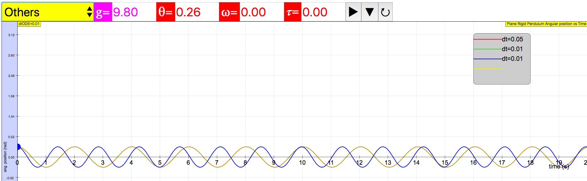
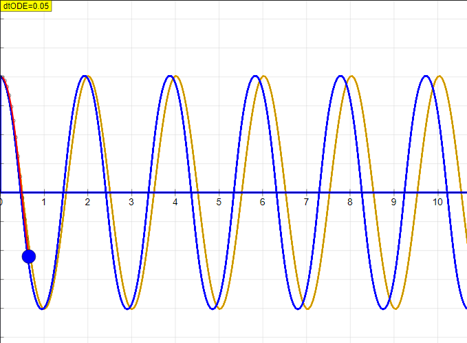
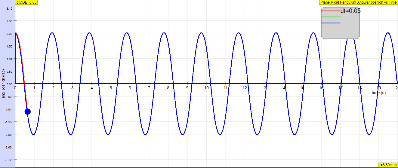
With a properly working model, and no exact solution with which to compare, the student should look for some kind of convergence behavior in the computational solution as Δt$\mathrm{\Delta }t$ is systematically made smaller. Figure 1 demonstrates this convergence behavior.

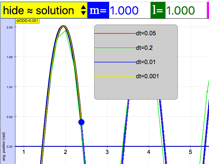
In EJSS, Using Runge Kutta 4 as solver, dt = 0.01 to 0.05 is an acceptable time step for accuracy.

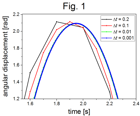
The parameters used to produce the computational solutions shown in figure 1 were: g=9.8 ms2,m=1.0 kg,L=1.0 m,b=0,ω=0,τd=0,θ0=120∘,θ0˙=0$g=9.8\frac{\text{m}}{{\text{s}}^2},m=1.0\text{kg},L=1.0\text{m},b=0,\omega =0,{\tau }_d=0,{\theta }_0={120}^{\circ },\dot{{\theta }_0}=0$. There a four curves in figure 1, that represent four different time steps. Lines are shown connecting the points that represent the discrete computational solutions. As Δt$\mathrm{\Delta }t$ is decreased the solution asymptotically approaches a specific shape and position. Upon close examination, one can just barely see the green dots (Δt=0.01$\mathrm{\Delta }t=0.01$) to the left of the blue curve (Δt=0.001$\mathrm{\Delta }t=0.001$). Reducing Δt$\mathrm{\Delta }t$ by the factor of ten from Δt=0.01$\mathrm{\Delta }t=0.01$ to Δt=0.001$\mathrm{\Delta }t=0.001$ does not produce a very significant change in the computational solution. Lowering Δt$\mathrm{\Delta }t$ even further may not produce a sufficient improvement in accuracy to be worth the extra computational time required.

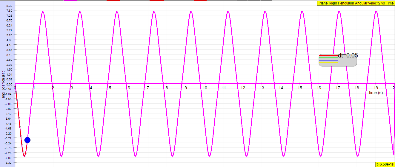
Figures 2 and 3 show the angular displacement and angular velocity, respectively, as a function of time for the parameters listed above, and Δt=0.001$\mathrm{\Delta }t=0.001$ s.

 

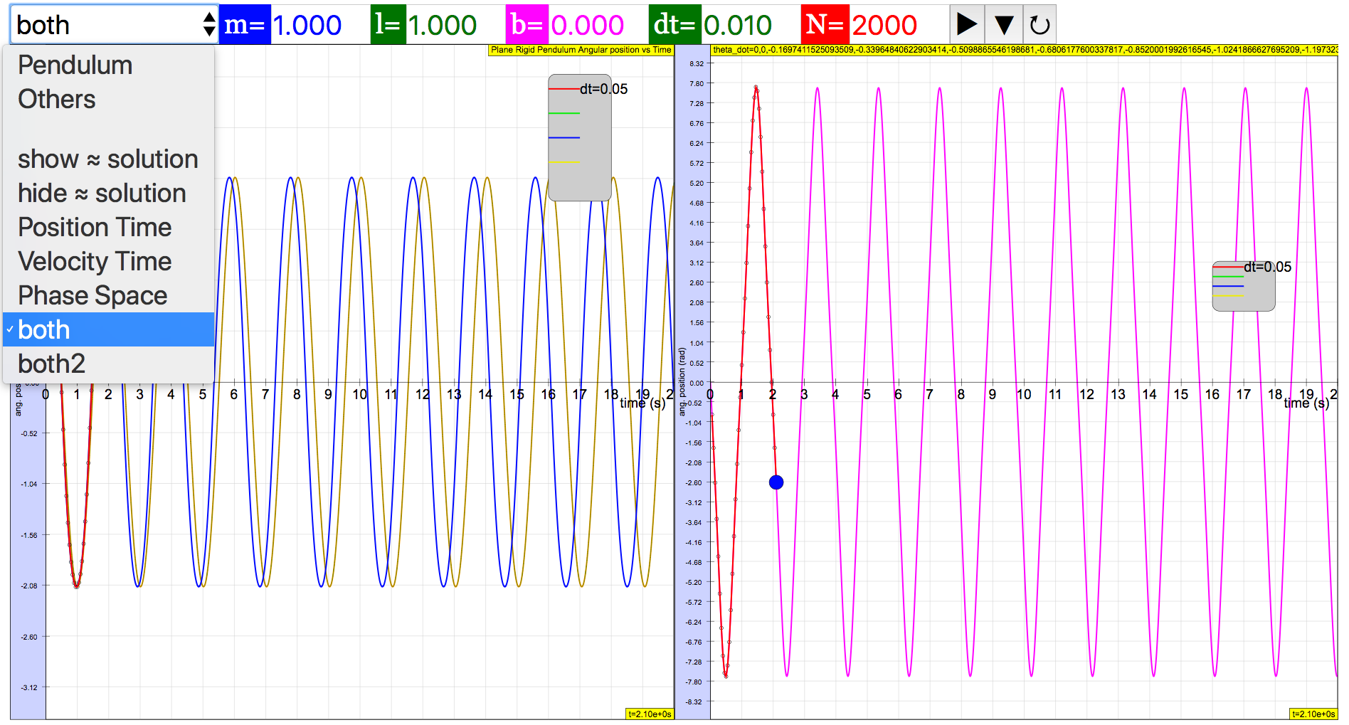
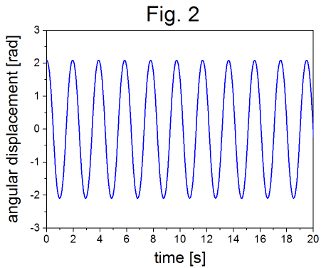
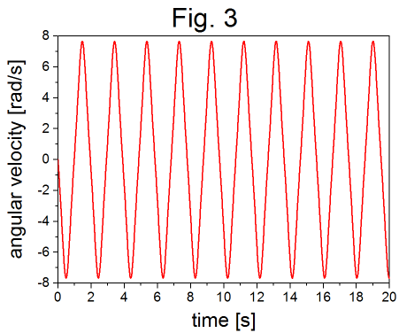
These graphs represent the oscillatory behavior of a pendulum. The angular velocity is 90∘${90}^{\circ }$ out of phase with the angular displacement, as expected.

The parameters used for these plots were:g=9.8 ms2,m=1.0 kg,L=1.0 m,b=0,ω=0,τd=0,θ0=120∘,θ0˙=0$g=9.8\frac{\text{m}}{{\text{s}}^2},m=1.0\text{kg},L=1.0\text{m},b=0,\omega =0,{\tau }_d=0,{\theta }_0={120}^{\circ },\dot{{\theta }_0}=0$.

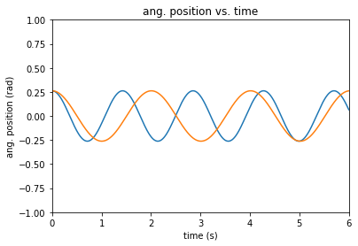
Exercise 2: Comparison with Analytical Small Angle Approximation Solution

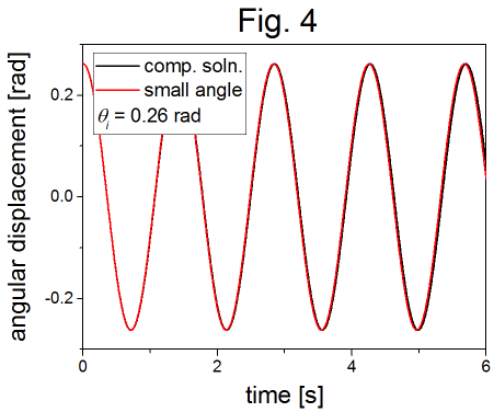
Figure 4 shows a comparison between the computational solution and the function

for the angular displacement in the small angle approximation. The parameters used were: g=9.8 ms2,m=1.0 kg,L=1.0 m,b=0,ω=0,τd=0,θ0=15∘,θ0˙=0,Δt=0.001 s$g=9.8\frac{\text{m}}{{\text{s}}^2},m=1.0\text{kg},L=1.0\text{m},b=0,\omega =0,{\tau }_d=0,{\theta }_0={15}^{\circ },\dot{{\theta }_0}=0,\mathrm{\Delta }t=0.001\text{s}$.

i speculate the suggested answers are wrong.

For an initial angular displacement of 0.26 radians (15∘${15}^{\circ }$), the computational solution matches the small angle approximation well until about the 3rd or 4th period. Figure 5 shows a zoomed-in view of the 4th maximum, showing that the difference between the two curves grows in time.

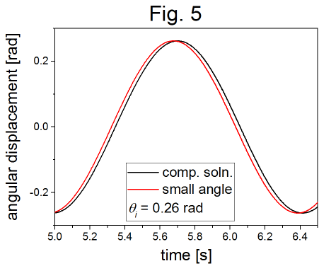
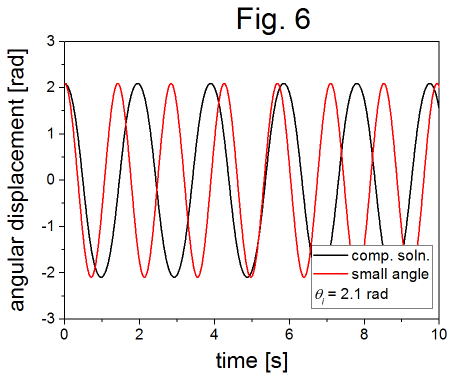
Figure 6 shows the same comparison for an initial angular displacement of 2.1 radians (120∘${120}^{\circ }$). There is a clear deviation between the computational solution and the small angle approximation observed at the outset. The small angle approximation underestimates the period of oscillation, and obviously isn’t a good approximation for large angles.

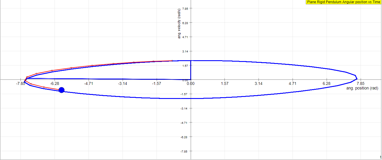
Exercise 3: Phase Space

Figure 7 shows a phase space plot (angular velocity vs. angular displacement) for three initial angular displacements, 0.26 rad (15∘${15}^{\circ }$), 1.3 rad (75∘${75}^{\circ }$), and 2.1 rad (120∘${120}^{\circ }$).

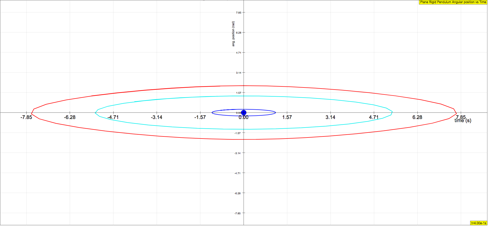
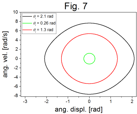
The parameters used for figure 7 were g=9.8 ms2,m=1.0 kg,L=1.0 m,b=0,ω=0,τd=0,θ0=120∘,θ0˙=0,Δt=0.001 s$g=9.8\frac{\text{m}}{{\text{s}}^2},m=1.0\text{kg},L=1.0\text{m},b=0,\omega =0,{\tau }_d=0,{\theta }_0={120}^{\circ },\dot{{\theta }_0}=0,\mathrm{\Delta }t=0.001\text{s}$. For the undamped, unforced SHO, the phase space trajectory is a well-defined closed path. It should also be emphasized that there is a direction of circulation around the closed orbit, the direction of which depends on the initial conditions.

Exercise 4: Damped Rigid Pendulum

Figure 8 shows the angular displacement and corresponding phase space plots for three different values of the damping strength, as labeled in the figure. The other parameters used were g=9.8 ms2,m=1.0 kg,L=1.0 m,ω=0,τd=0,θ0=120∘,θ0˙=0,Δt=0.001 s$g=9.8\frac{\text{m}}{{\text{s}}^2},m=1.0\text{kg},L=1.0\text{m},\omega =0,{\tau }_d=0,{\theta }_0={120}^{\circ },\dot{{\theta }_0}=0,\mathrm{\Delta }t=0.001\text{s}$.

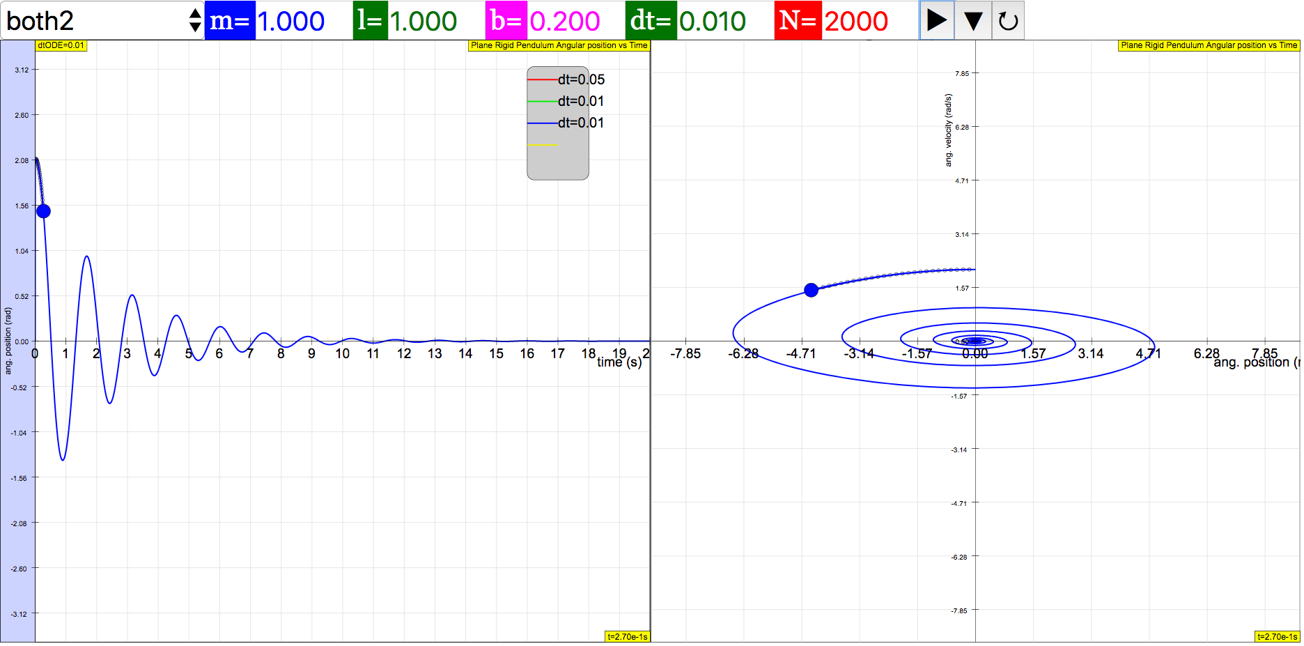
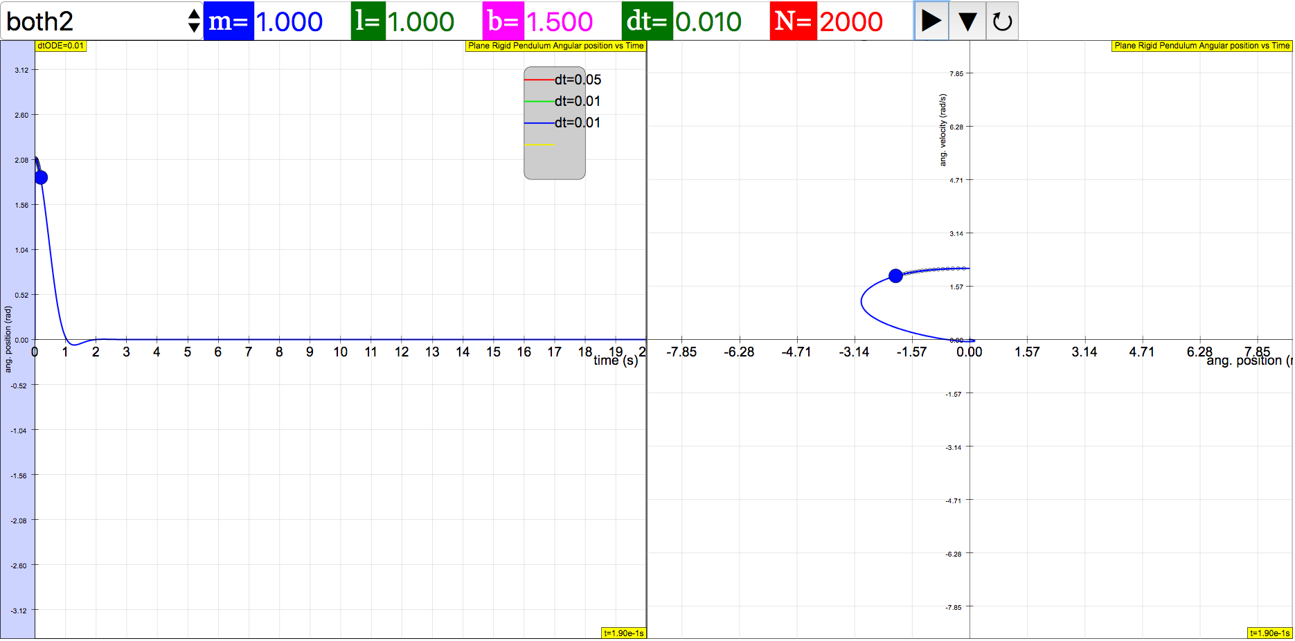
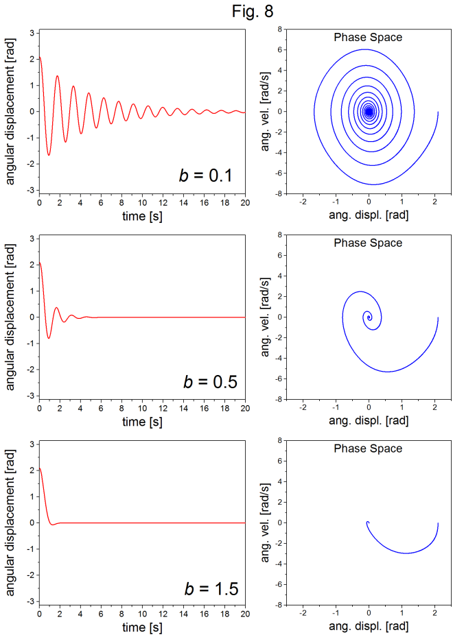
As expected, the oscillations become damped, and the corresponding phase space trajectory spirals in towards zero as the energy approaches complete dissipation. For a value of roughly b=1.5 kgm2s$b=1.5\frac{\text{kg}{\text{m}}^2}{s}$ and above, there are no longer oscillatory solutions.

Exercise 5: Damped, Driven Rigid Pendulum

Figure 9 shows shows the angular displacement and corresponding phase space plots for three different values of the driving torque as labeled in the figure. The other parameters used were g=9.8 ms2,m=1.0 kg,L=1.0 m,b=0.2 kgm2s,ω=3.0 rad/s,θ0=120∘,θ0˙=0,Δt=0.001 s$g=9.8\frac{\text{m}}{{\text{s}}^2},m=1.0\text{kg},L=1.0\text{m},b=0.2\frac{\text{kg}{\text{m}}^2}{s},\omega =3.0\text{rad/s},{\theta }_0={120}^{\circ },\dot{{\theta }_0}=0,\mathrm{\Delta }t=0.001\text{s}$. The phase space plots were generated with 200,000 time steps.

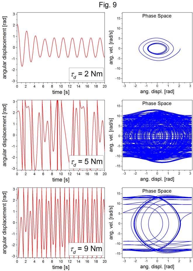
For the lowest value of the driving torque, after the transient response, the system settles into predictable oscillatory behavior, and a well defined elliptical orbit in phase space. But, with higher driving torques, the system shows an apparently unpredictable non-repeating oscillatory behavior, with the corresponding phase space characterized by many orbits that can appear, as the case of τd=5 Nm${\tau }_d=5\text{Nm}$, to be completely random. This behavior is chaotic.

Though chaos identification is beyond the scope of this exercise set, the phase space results of Exercise 5 provide a good opportunity to demonstrate to students the chaotic coincidental nature of deterministic solutions and unpredictability.

 

Translations

Code	Language		Translator	Run

Credits

Fremont Teng; Loo Kang Wee; based on python codes by K. Roos

Sample Learning Goals

[text]

For Teachers

Plane Rigid Pendulum JavaScript Simulation Applet HTML5

Instructions

Combo Box and Functions

Toggling Full Screen

Play/Pause, Initialise and Reset Buttons

Research

[text]

Video

[text]

 Version:

1. https://www.compadre.org/PICUP/exercises/exercise.cfm?I=139&A=RigPend 
2. http://weelookang.blogspot.com/2018/06/plane-rigid-pendulum-javascript.html 

Other Resources

[text]