About

Subject Area	Mechanics
Levels	First Year and Beyond the First Year
Available Implementations	C/C++, Fortran, IPython/Jupyter Notebook, Mathematica, Octave*/MATLAB, Python, and Spreadsheet
Learning Objectives	Students who complete this set of exercises will be able to build a model of a simple hanging harmonic oscillator using the Euler algorithm (Exercises 1 and 2); be able to build a model of a simple hanging harmonic oscillator using the Euler-Cromer algorithm (Exercises 4 and 5); be able to produce graphs of the positon, velocity, and total energy as a function of time from the results of their computational model (Exercises 1-5); be able to assess the accuracy of two different computational algorithms (Euler and Euler-Cromer) by comparing results from the different algorithms to each other and to the exact analytical solution (Exercises 1-5); discover that they bloody well can’t use the simple Euler method when modeling an oscillatory system (Exercises 1-3).

# Written by:

# Kelly Roos

# Engineering Physics

# Bradley University

# rooster@bradley.edu | 309.677.2997

import numpy as np

import matplotlib.pyplot as plt

import math

# Input parameters for model

dt = 0.01 # time step (s)

vi = 0 # initial velocity (m/s)

yi = 0.1 # initial position (m), relative to eq position yeq (m)

m = 1.0 # mass (kg)

g = 9.8 # gravity (m/s^2)

k = 10 # spring constant (N/m)

t_steps = 2000 # number of time steps

# Defines the 1D arrays to be used in the computation and

# sets all values in the arrays to zero

time = np.zeros(t_steps)

y_Euler = np.zeros(t_steps)

y_EC = np.zeros(t_steps)

y_exact = np.zeros(t_steps)

v_Euler = np.zeros(t_steps)

v_EC = np.zeros(t_steps)

v_exact = np.zeros(t_steps)

energyEuler = np.zeros(t_steps);

energyEC = np.zeros(t_steps);

# Initial conditions

time[1] = 0

y_Euler[1] = yi

y_EC[1] = yi

y_exact[1] = yi

v_Euler[1] = vi

v_EC[1] = vi

v_exact[1] = vi

energyEuler[1]=0.5*m*v_Euler[1]**2+0.5*k*(y_Euler[1]+m*g/k)**2-m*g*(y_Euler[1]+m*g/k)

energyEC[1]=0.5*m*v_EC[1]**2+0.5*k*(y_EC[1]+m*g/k)**2-m*g*(y_EC[1]+m*g/k)

# Main loop: Euler algorithm, euler-Cromer, and evaluation of exact solutions for v and y

for i in range(2, t_steps):

time[i] = time[i-1] + dt

# Euler

v_Euler[i]=v_Euler[i-1]-k*y_Euler[i-1]*dt/m

y_Euler[i]=y_Euler[i-1]+v_Euler[i-1]*dt

# Euler-Cromer

v_EC[i]=v_EC[i-1]-k*y_EC[i-1]*dt/m

y_EC[i]=y_EC[i-1]+v_EC[i]*dt

# Exact (assuming vi=0)

v_exact[i]=-yi*math.sqrt(k/m)*math.sin(math.sqrt(k/m)*time[i])

y_exact[i]=yi*math.cos(math.sqrt(k/m)*time[i])

# Energies

energyEuler[i]=0.5*m*v_Euler[i]**2+0.5*k*(y_Euler[i]+m*g/k)**2-m*g*(y_Euler[i]+m*g/k)

energyEC[i]=0.5*m*v_EC[i]**2+0.5*k*(y_EC[i]+m*g/k)**2-m*g*(y_EC[i]+m*g/k)

# Plotting Results

plt.plot(time, v_Euler, time, v_EC)

plt.ylim((-0.3, 0.3))

plt.xlim((0, 20))

plt.xlabel('time (s)')

plt.ylabel('position (m)')

plt.title('position vs. time')

plt.show()

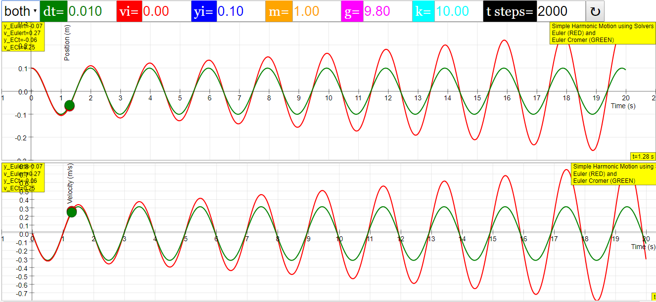
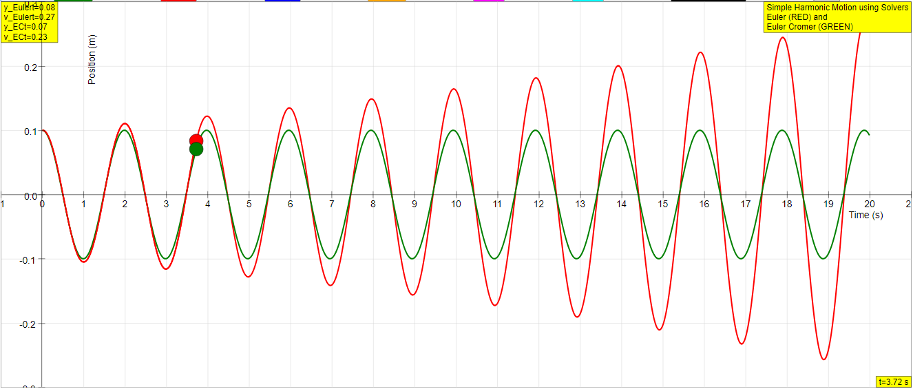
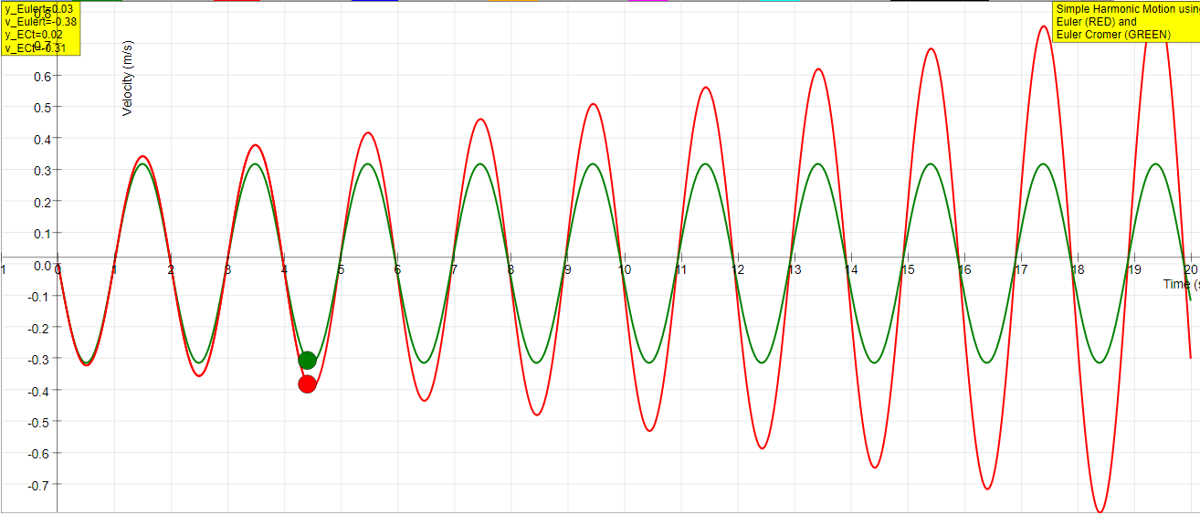
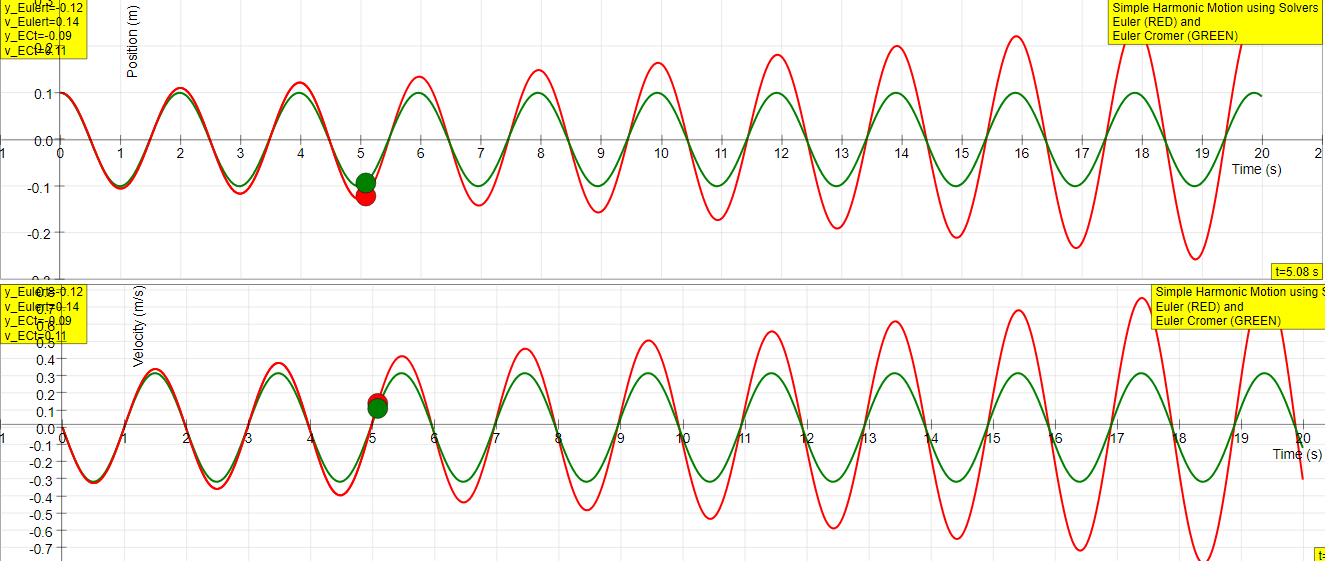
Exercise 1: Euler Algorithm Model of a SHO

Build a computational model of a simple hanging harmonic oscillator using the Euler method. Use realistic values for the parameters (i.e., spring constant k and attached mass m, such as would be encountered in a typical introductory mechanics laboratory exercise. Also, assume that the mass of the spring is negligible compared to the attached mass, and that the harmonic oscillator has been stretched vertically downward a distance y0, relative to its hanging equilibrium position and released from rest. Use the model to produce graphs of the position and velocity of the mass as a function of time, and compare these with the exact functions for the position and velocity,

and

that result from solving Newton’s 2nd Law analytically. Does the angular frequency match that expected for a simple harmonic oscillator of mass m an spring constant k?

Exercise 2: Artificial Behavior with the Euler Algorithm

You may (should!) have noticed that something is not right with the Euler model of your hanging oscillator. Describe in detail the artificial behavior you observe in your model, and explain why it doesn’t represent a realistic oscillating mass. Recall that in the Euler method, the accuracy of the solution can be increased by using a smaller value of Δt. Can you get rid of the artificial behavior by making Δt smaller?

Exercise 3: Energy in the Euler Algorithm Model of a SHO

Modify your model to produce a graph of the total energy of the oscillator as a function of time. Describe in detail what happens to the energy, and the artificial behavior observed. Can this artificial behavior in the energy be corrected by making Δt smaller? What can you conclude about using the Euler method to model a simple harmonic oscillator?

Exercise 4: Euler-Cromer Algorithm Model of a SHO

Build a model of the hanging oscillator using the modified Euler, or Euler-Cromer, numerical method. Compare the results you obtain (i.e. position and velocity vs. time) with those obtained from the simple Euler method, and with the exact solution. Comment in detail on your results.

Exercise 5: Energy in the Euler-Cromer Algorithm Model of a SHO

Modify your model to produce a graph of the total energy as a function of time. Is energy conserved for the Euler-Cromer algorithm?

 

Translations

Code	Language		Translator	Run

Credits

Fremont Teng; Loo Kang Wee

1. Overview:

This document reviews the key information presented in the provided excerpts from the Open Educational Resources / Open Source Physics @ Singapore website, specifically focusing on their "PICUP Hanging Simple Harmonic Oscillator JavaScript Simulation Applet HTML5." The resource offers a set of exercises designed to teach students about computational modeling of a physical system, specifically a hanging mass-spring oscillator, using numerical methods. A core objective is to highlight the limitations of the simple Euler algorithm for oscillatory systems and to introduce the more stable Euler-Cromer algorithm.

2. Main Themes and Important Ideas/Facts:

• Computational Modeling of a Simple Harmonic Oscillator (SHO): The central theme is the construction and analysis of computational models of a hanging mass-spring system constrained to one-dimensional motion. This involves using numerical methods to approximate the system's behavior over time.
• Introduction to Numerical Methods: The resource explicitly focuses on two numerical methods: the simple Euler algorithm and the Euler-Cromer algorithm. These are used to discretize time and iteratively calculate the position and velocity of the mass.
• Limitations of the Euler Algorithm for Oscillatory Systems: A critical finding intended for students is that the simple Euler method exhibits "artificial behavior" when modeling oscillatory systems, particularly the non-conservation of energy. The exercises guide students to "discover that they bloody well can’t use the simple Euler method when modeling an oscillatory system."
• Necessity of the Euler-Cromer Algorithm: The resource introduces the Euler-Cromer algorithm as a modification of the Euler method that is more suitable for modeling oscillatory systems because it avoids the artificial energy dissipation seen with the simple Euler method. The exercises encourage students to compare the results of both algorithms.
• Importance of Energy Conservation in Physical Models: The exercises emphasize the concept of energy conservation in a simple harmonic oscillator. Students are tasked with plotting the total energy of the system over time for both algorithms and comparing it to the expected behavior.
• Comparison with Analytical Solutions: The exercises require students to compare the results obtained from their computational models (using both Euler and Euler-Cromer) with the "exact analytical solution" for the position and velocity of the mass. This allows them to assess the accuracy of the numerical methods.
• Hands-on Learning and Discovery: The structure of the resource is based on a series of guided exercises where students actively build and analyze their own computational models. This promotes a "discover[y]" learning approach.
• Available Implementations: The resource notes that the exercises can be implemented in various programming environments, including "C/C++, Fortran, IPython/Jupyter Notebook, Mathematica, Octave*/MATLAB, Python, and Spreadsheet," indicating flexibility for different educational settings. The provided code snippet is in Python.
• Learning Objectives: The stated learning objectives clearly outline what students should be able to do upon completing the exercises, including building models with both algorithms, producing graphs of motion and energy, assessing the accuracy of the algorithms, and understanding the limitations of the Euler method for oscillatory systems.

3. Key Quotes and Analysis:

• "the Euler algorithm does not conserve energy, and that for this simple oscillatory system, a modified algorithm (Euler-Cromer) is necessary to avoid artificial behavior in the model." This quote succinctly summarizes the core finding and the rationale for introducing the Euler-Cromer method. It highlights the fundamental flaw of the simple Euler method in this context.
• "discover that they bloody well can’t use the simple Euler method when modeling an oscillatory system ( Exercises 1-3 )." This informal but emphatic statement underscores the intended learning outcome regarding the unsuitability of the Euler method for SHOs.
• The provided Python code snippet demonstrates the implementation of both the Euler and Euler-Cromer algorithms for a hanging SHO. It includes parameters like time step (dt), initial conditions (vi, yi), mass (m), gravity (g), spring constant (k), and the main loop where the numerical updates for position and velocity are calculated. The code also includes the calculation of energy for both methods and the plotting of the results.
• The analytical solutions provided for position and velocity:
• y ( t ) = y 0 cos (t* √(k/m) ) (1)
• v ( t ) = − √(k/m)* y 0 sin ( √(k/m)* t ) , (2) These equations serve as the benchmark against which the numerical solutions are compared, allowing students to evaluate the accuracy of the Euler and Euler-Cromer methods.
• The learning objectives such as "be able to assess the accuracy of two different computational algorithms (Euler and Euler-Cromer) by comparing results from the different algorithms to each other and to the exact analytical solution ( Exercises 1-5 )" and "be able to produce graphs of the positon, velocity, and total energy as a function of time from the results of their computational model ( Exercises 1-5 )" clearly indicate the active learning and analytical skills the resource aims to develop.

4. Implications and Potential Uses:

This resource appears to be a valuable tool for introductory physics courses, particularly those incorporating computational methods. It allows students to gain a deeper understanding of:

• The principles of simple harmonic motion.
• The concept of energy conservation in physical systems.
• The basics of numerical modeling and the challenges associated with different numerical algorithms.
• The importance of choosing appropriate numerical methods for specific types of physical problems.

The availability of the exercises in multiple programming languages makes it adaptable to various curricula and student backgrounds. The guided discovery approach can be highly effective in promoting conceptual understanding and critical thinking about the limitations and strengths of computational modeling techniques.

5. Further Considerations:

• The level of mathematical and programming background assumed for students undertaking these exercises would be an important factor to consider for educators.
• The "Intro Page" and the specifics of "Exercises 1-5" (beyond the titles) would provide further detail on the pedagogical approach and the specific tasks involved for the students.
• The JavaScript Simulation Applet mentioned in the title, but not detailed in the excerpts, likely provides an interactive environment for students to explore the behavior of the hanging SHO with different parameters and algorithms.

This briefing document provides a comprehensive overview of the main themes and important aspects of the PICUP Hanging Simple Harmonic Oscillator resource based on the provided excerpts. It highlights the educational goals, the methods employed, and the key takeaways for students engaging with this material.

 

Study Guide: Computational Modeling of a Hanging Simple Harmonic Oscillator

Key Concepts

• Simple Harmonic Oscillator (SHO): A system that, when displaced from its equilibrium position, experiences a restoring force proportional to the displacement. This results in oscillatory motion.
• Hanging Mass-Spring System: A specific type of SHO where a mass is attached to a spring and hangs vertically under the influence of gravity and the spring force.
• Newton's Second Law: The net force acting on an object is equal to the mass of the object multiplied by its acceleration (F = ma).
• Computational Model: A mathematical representation of a system that is implemented using numerical algorithms to simulate its behavior over time.
• Euler Algorithm: A first-order numerical method for approximating the solution of ordinary differential equations. It uses the current value to estimate the value at the next time step.
• Euler-Cromer Algorithm: A modification of the Euler algorithm often used for oscillatory systems. It updates the velocity using the force at the current time step and then uses the updated velocity to find the position at the next time step.
• Time Step (Δt or dt): The discrete intervals of time used in a computational model to advance the simulation.
• Position (y): The location of the mass relative to a reference point (in this case, often the equilibrium position).
• Velocity (v): The rate of change of position with respect to time.
• Energy Conservation: In an ideal isolated system, the total energy (sum of kinetic and potential energy) remains constant over time.
• Artificial Behavior: Unphysical or inaccurate results in a computational model that arise from the limitations of the numerical method rather than the physics of the system.
• Exact Analytical Solution: The precise mathematical solution to the equations of motion, derived without approximations.
• Angular Frequency (ω): A measure of the rate of oscillation, related to the frequency (f) by ω = 2πf and to the mass (m) and spring constant (k) of a SHO by ω = √(k/m).
• Kinetic Energy: The energy of motion, given by (1/2)mv².
• Potential Energy (Spring): The energy stored in a spring due to its compression or extension, given by (1/2)k(Δy)², where Δy is the displacement from the equilibrium position.
• Potential Energy (Gravitational): The energy an object possesses due to its position in a gravitational field, given by mgh (in this 1D case, relative to a chosen zero point). In the context of the provided code, the potential energy term includes both spring and gravitational contributions relative to a defined equilibrium.

Quiz

1. What is the primary goal of the exercises described in the source material?
2. Briefly explain the fundamental difference between the Euler and Euler-Cromer algorithms as applied to modeling the hanging simple harmonic oscillator.
3. According to the source, what is a significant limitation of using the simple Euler method for modeling oscillatory systems like a hanging mass-spring?
4. What quantities are typically plotted as a function of time when analyzing the behavior of the hanging simple harmonic oscillator in these exercises?
5. Why is it important to compare the results of a computational model with the exact analytical solution when one is available?
6. In the context of the hanging simple harmonic oscillator, what causes the restoring force that leads to oscillations?
7. What does the Euler-Cromer algorithm do differently in updating the position compared to the Euler algorithm, and why is this often beneficial for oscillatory systems?
8. What is meant by "artificial behavior" in the context of these computational models, and what is one example of such behavior observed with the Euler method?
9. How does the total energy of the system behave over time when modeled using the Euler algorithm, according to the source?
10. What conclusion does the source material suggest regarding the suitability of the simple Euler method for modeling a simple harmonic oscillator?

Quiz Answer Key

1. The primary goal is for students to build computational models of a hanging mass-spring system using the Euler and Euler-Cromer numerical schemes and to understand the accuracy and limitations of these methods by comparing their results to each other and to the exact analytical solution.
2. The Euler algorithm uses the velocity at the current time step to update the position at the next time step, while the Euler-Cromer algorithm uses the velocity at the next time step (calculated using the force at the current time) to update the position at the next time step.
3. A significant limitation of the simple Euler method is that it does not conserve energy when modeling oscillatory systems, leading to artificial behavior where the amplitude of oscillations may grow or decay unrealistically over time.
4. The quantities typically plotted as a function of time are the position of the mass, the velocity of the mass, and the total energy of the oscillator.
5. Comparing computational results with the exact analytical solution allows for an assessment of the accuracy of the numerical algorithm and helps to identify any artificial behavior or discrepancies introduced by the approximation methods.
6. The restoring force in a hanging simple harmonic oscillator is due to the combination of the spring force (proportional to the displacement from equilibrium) and the force of gravity (which shifts the equilibrium position but contributes to the oscillation around it).
7. The Euler-Cromer algorithm updates the position using the newly calculated velocity at the next time step, whereas the Euler algorithm uses the velocity from the current time step. This seemingly small change often leads to better energy conservation in oscillatory systems.
8. "Artificial behavior" refers to non-physical or inaccurate results produced by the computational model due to the numerical method itself. An example with the Euler method is the increasing amplitude of oscillations over time, which violates energy conservation.
9. When modeled with the Euler algorithm, the total energy of the oscillator typically increases over time, indicating a non-physical addition of energy to the system and contributing to the artificial growth in oscillation amplitude.
10. The source material strongly suggests that the simple Euler method is not suitable for accurately modeling a simple harmonic oscillator due to its failure to conserve energy and the resulting artificial behavior, particularly over longer simulation times.

Essay Format Questions

1. Discuss the fundamental differences between the Euler and Euler-Cromer algorithms and explain why the Euler-Cromer method is generally more suitable for modeling oscillatory systems like the hanging simple harmonic oscillator. Support your explanation by referring to the concepts of energy conservation and artificial behavior.
2. Analyze the artificial behavior that arises when modeling a simple harmonic oscillator using the Euler algorithm. Describe the characteristics of this behavior in terms of position, velocity, and total energy, and discuss why reducing the time step (Δt) may not completely eliminate these inaccuracies.
3. The exercises emphasize the importance of comparing computational models with exact analytical solutions. Explain why this comparison is crucial in assessing the validity and accuracy of numerical methods. Discuss what can be learned by observing discrepancies between the two approaches in the context of a hanging simple harmonic oscillator.
4. Consider the learning objectives outlined in the source material. Describe how building and analyzing computational models of a hanging simple harmonic oscillator using both the Euler and Euler-Cromer algorithms can help students develop a deeper understanding of numerical methods, energy conservation, and the limitations of approximations in physics.
5. Based on the provided information, evaluate the statement: "The Euler method is a universally applicable numerical technique for solving equations of motion in physics." Use the example of the simple harmonic oscillator to support your argument for or against this statement, and propose alternative or modified approaches when dealing with oscillatory systems.

Glossary of Key Terms

• Algorithm: A set of well-defined instructions for performing a task or solving a problem, often used in computation.
• Computational Model: A mathematical representation of a real-world system that is implemented using software to simulate its behavior.
• Differential Equation: An equation that relates a function with its derivatives, often describing the rates of change in physical systems.
• Equilibrium Position: The position where the net force on an object is zero, and the object remains at rest if placed there.
• Numerical Method: An approximate technique for finding solutions to mathematical problems, often involving iterative calculations.
• Oscillation: A repetitive variation, typically in time, of some measure about a central value or between two or more different states.
• Restoring Force: A force that acts to return a system to its equilibrium position after it has been displaced.
• Simulation: The process of using a model to study the behavior of a system over time, often involving numerical computation.
• Spring Constant (k): A measure of the stiffness of a spring, defined as the force required to stretch or compress the spring by a unit length.
• Total Energy: The sum of all forms of energy in a system, such as kinetic energy and potential energy.

Sample Learning Goals

[text]

For Teachers

Hanging Simple Harmonic Oscillator JavaScript Simulation Applet HTML5

Instructions

Graph Combo Box

Control Panel

Reset Button

Research

[text]

Video

[text]

 Version:

1. https://www.compadre.org/PICUP/exercises/exercise.cfm?I=135&A=SHHO 
2.  http://weelookang.blogspot.com/2018/05/hanging-simple-harmonic-oscillator.html

Other Resources

[text]