About

The Superposition Principle

The fundamental building blocks of one-dimensional quantum mechanics are energy eigenfunctions ψ_n(x) and energy eigenvalues E_n. For a given potential energy function V(x) and boundary conditions, energy eigenfunctions can be determined either analytically or numerically. Most of the time in quantum mechanics these energy eigenfunctions are determined in position space. Once these energy eigenstates are determined, more interesting quantum-mechanical wave functions Ψ(x,t) can be studied by applying the superposition principle

where the expansion coefficients c_n satisfy Σ c_n|² = 1. Depending on how many of the coefficients c_n are non-zero, one may have an energy eigenstate, a two-state superposition, or even an initially localized (usually Gaussian shaped) wave packet.

Any complete orthonormal set of eigenfunctions can be used to construct the wave function Ψ(x,t). This simulation uses the superposition principle to construct and display a time-dependent wave function using either infinite square well (ISW) or simple harmonic oscillator (SHO) eigenfunctions.

Units

Although the metric (MKS) system of units has become the standard international system of units, it is not well suited for computation if the quantities being computed are very large or very small. Quantum phenomena occurs on the microscopic scale at very fast times and computations are usually done using an atomic system of units in which the reduced Plank's constant ħ, the Bohr radius a_o, and the mass of the electron m are set equal to unity. The one-dimensional time independent Schrödinger equation in these units is:

In atomic units, one unit time is 2.42×10^-17 seconds, one unit of distance is 5.29×10^-11 meters, and one unit of energy is 4.36×10^-18 Joules. This simulation models a particle with the mass of an electron using these atomic units.

References:

• For an excellent tutorial on energy eigenfunction shape and the relationship to the potential energy function, see: A. P. French and E. F. Taylor, Qualitative plots of bound state wave functions, Am. J. Phys. 39, 961-962 (1971).
• An Introduction to Quantum Mechanics (2ed) by David J. Griffiths page 28.

Credits:

The Bound Energy Eigenstate Superposition JavaScript simulation was developed by Wolfgang Chrsitian using the Easy Java/JavaScript Simulations (EjsS) modeling tool. You can examine and modify this simulation if you have EjsS version 5.2 or above installed by importing the model's zip archive into EjsS. Information about EjsS is available at: <http://www.um.es/fem/Ejs/> and in the OSP ComPADRE collection <http://www.compadre.org/OSP/>.

The following Options cannot work on SHO (but works if system=ISO):

-"SHO squeezed"

-"SHO squeezed wide"

-"SHO boosted coherent"

-"SHO boosted squeezed"

-"SHO shifted ground state"

-"SHO shifted excited state"

Infinite Square Well Exercises

[Screen shot of an ISW superposition state that as it hits one side of the well.]

Pre-set Demonstrations

You can access the pre-set initial states for the infinite square well (ISW) via the textbox on the lower-left-hand side of the main simulation panel.  These show:

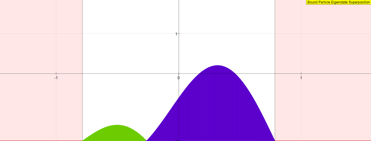
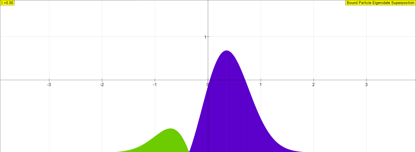
• ISW Two State: Loads an ISW two-state superposition (equal mix of ground state and first-excited state).
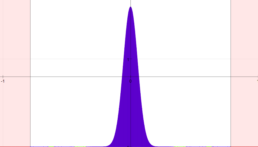
• ISW Gaussian: Loads an ISW initial Gaussian wave packet with no initial average momentum.
• ISW Narrow Gaussian <p>₀ = 0: Loads an ISW initial Gaussian wave packet with no initial average momentum.
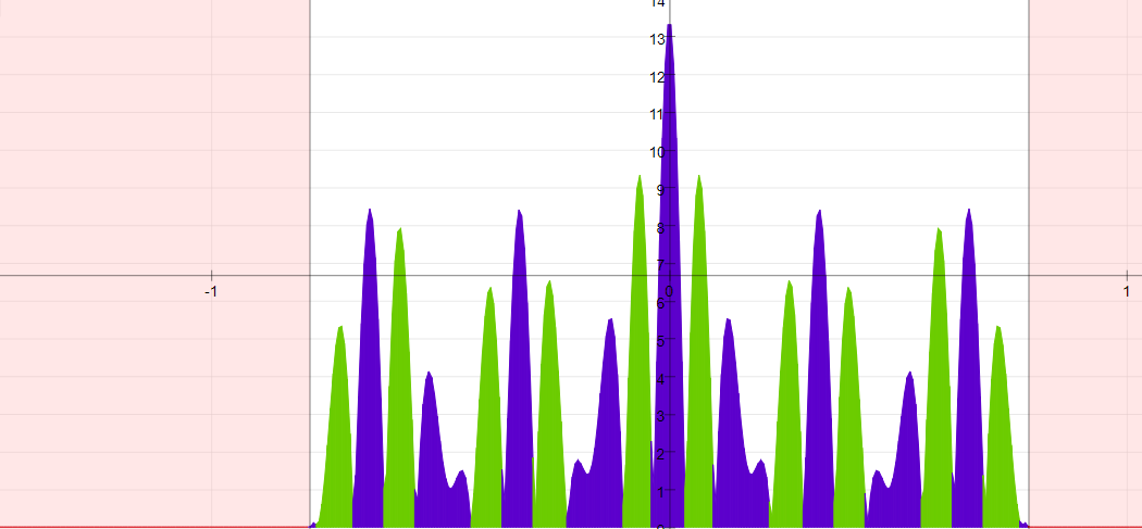
• ISW Narrow Gaussian <p>₀ = 80 π/a: Loads an ISW initial Gaussian wave packet with an initial average momentum.

Exercises

1. Given the default infinite square well width of a = 1.57 = π/2, what are the ground-state and first-excited-state energies?  Recall that we have scaled the problem such that ħ = m = 1.

2. Since the time dependence of energy eigenstates is just, e^-iEnt/ħ, how long does it take the ground state and the first-excited state to evolve in time back to their t = 0 values? In other words, with what period do these states oscillate with time? Once you have these values compare them to each other.

3. Now select the ISW Two State and set the dt to the ground state period divided by 10.  The text field can accept simple mathematical operations such as /, *, pi, etc. Single step through the simulation and see if the wave function indeed has the same period as you calculated in Question 2.  Now set the dt to the ground state period divided by 3 and run the simulation. Single step through the simulation and describe the the wave function at these times. Why does this occur? What odes this result mean for the period of expectation values of x, <x>?

4. Now select one of the ISW Gaussian wave packets (ISW Gaussian, ISW Narrow Gaussian <p>0 = 0, ISW Narrow Gaussian <p>0 = 80 π/a) from the drop down menu. First look at all three wave packets. Describe the similarities and differences between the packets' initial shapes. Choose one packet and set the dt to the ground state period divided by 100 and run the simulation. Describe the motion of each wave packet. Which packet initially behaves like a particle in a classical infinite square well?

5. Now set the dt to the ground state period divided by 10 and single step through the simulation. What do you notice about the wave function at these times? Now set dt to the ground state period divided by 4, then 3 and single step through the simulation. Again describe what do you notice about the wave function at these times.

Infinite Square Well Eigenfunctions

[Screen shot of the energy eigenfunction describing the ISW first-excited state.]

The infinite square well (ISW) is an idealized model consisting of a point mass m inside an infinitely deep well of width a.  According to quantum mechanics, the energy eigenfunctions ψ_n(x) for a symmetric ISW are simple sinusoidal functions
 

.

The corresponding energy eigenvalues E_n scale as the principal quantum number n squared

 

.

Simple Harmonic Oscillator Eigenfunctions

[Screen shot of the SHO ground state.]

A simple harmonic oscillator (SHO) with a potential energy V(x) = ½mω²x²   has energy eigenfunctions ψ_n(x) that are expressed in terms of a Gaussian times a Hermite polynomial H_n(x)
 

 

The angular frequency ω=(K/m)^½ is that of a classical mass on a spring with spring constant K.  Substituting these SHO eigenfunctions ψ_n(x) into the time-independent Schrödinger equation shows that they have energy eigenvalues E_n that scale as the principal quantum number n
 

.

 

Note that unlike the infinite square well model, the simple harmonic oscillator energy eigenvalues are evenly spaced.

 

In order to compare ISW and SHO eigenfunctions, the spring constant is chosen so that the ground state energy eigenvalues of these two systems are equal.

 

Translations

Code	Language		Translator	Run

Credits

Wolfgang Christian; Mario Belloni; Dieter Roess; Fremont Teng; Loo Kang Wee

Overview

This briefing document reviews the "Bound Eigenstate Superposition JavaScript Simulation Applet HTML5" resource available on the Open Educational Resources / Open Source Physics @ Singapore website. This interactive simulation is designed to help users understand the fundamental concept of superposition in one-dimensional quantum mechanics, specifically focusing on bound energy eigenstates within Infinite Square Well (ISW) and Simple Harmonic Oscillator (SHO) potentials. The resource provides a description of the underlying principles, explains the simulation's functionality, offers pre-set demonstrations, and includes exercises for deeper engagement with the concepts.

Main Themes and Important Ideas/Facts

1. The Superposition Principle:

• The core concept explored is the superposition principle in quantum mechanics.
• The resource states: "The fundamental building blocks of one-dimensional quantum mechanics are energy eigenfunctions ψn(x) and energy eigenvalues En... more interesting quantum-mechanical wave functions Ψ(x,t) can be studied by applying the superposition principle Ψ(x,t) = Σ cn ψn(x) e-i En t /ħ where the expansion coefficients cn satisfy Σ |cn|2 = 1."
• This principle allows for the construction of complex, time-dependent wave functions (Ψ(x,t)) by linearly combining energy eigenfunctions (ψn(x)) with specific coefficients (cn) and their corresponding time evolution (e-i En t /ħ).
• The number of non-zero coefficients determines the nature of the superposition, ranging from a single energy eigenstate to a multi-state superposition or a localized wave packet.
• The simulation utilizes the superposition principle to visualize the time evolution of wave functions constructed from the eigenfunctions of the Infinite Square Well (ISW) and the Simple Harmonic Oscillator (SHO).

2. Energy Eigenfunctions and Eigenvalues:

• The resource highlights that energy eigenfunctions (ψn(x)) and their corresponding energy eigenvalues (En) are fundamental to quantum mechanics for a given potential energy function V(x) and boundary conditions.
• These eigenfunctions are typically determined in position space.
• The simulation allows users to explore superpositions built from the eigenfunctions of two specific potential wells:
• Infinite Square Well (ISW): The eigenfunctions are described as "simple sinusoidal functions" and the energy eigenvalues "scale as the principal quantum number n squared."
• Simple Harmonic Oscillator (SHO): The eigenfunctions involve a "Gaussian times a Hermite polynomial Hn(x)" and the energy eigenvalues "scale as the principal quantum number n," being "evenly spaced."
• The resource notes that "In order to compare ISW and SHO eigenfunctions, the spring constant is chosen so that the ground state energy eigenvalues of these two systems are equal."

3. Atomic Units:

• The simulation employs atomic units for computational convenience at the microscopic scale.
• The resource explains: "Quantum phenomena occurs on the microscopic scale at very fast times and computations are usually done using an atomic system of units in which the reduced Plank's constant ħ, the Bohr radius ao, and the mass of the electron m are set equal to unity."
• The conversion factors to SI units are provided: "one unit time is 2.42×10-17 seconds, one unit of distance is 5.29×10-11 meters, and one unit of energy is 4.36×10-18 Joules."
• The simulation models a particle with the mass of an electron using these atomic units.

4. Simulation Functionality:

• The simulation, developed using the Easy Java/JavaScript Simulations (EjsS) tool, allows users to construct and visualize time-dependent wave functions.
• It provides controls to adjust parameters like time evolution (dt) and the width of the bounded region (for ISW).
• Users can select from pre-set initial states for the ISW, including:
• ISW Two State: Equal mix of ground and first excited states.
• ISW Gaussian: Initial Gaussian wave packet with no initial average momentum (various widths).
• ISW Narrow Gaussian
• 0 = 80 π/a: Gaussian wave packet with initial average momentum.
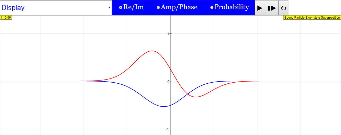
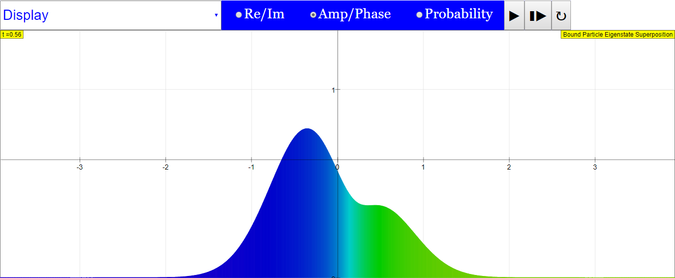
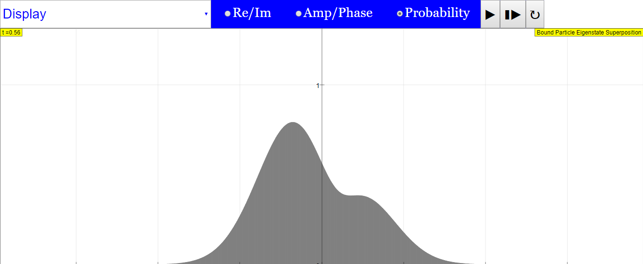
• The interface includes options to display different representations of the wave function (Re/Im, Amp/Phase, Probability).
• The simulation has play/pause, step, and reset buttons for controlling the animation.

5. Interactive Exercises (Infinite Square Well):

• The resource includes a set of exercises designed to guide users in exploring the behavior of superpositions within an infinite square well.
• These exercises involve:
• Calculating ground and first-excited state energies.
• Determining the oscillation periods of energy eigenstates.
• Observing the time evolution of a two-state superposition.
• Investigating the motion of Gaussian wave packets with different initial conditions and time steps.
• Analyzing the implications for the period of expectation values like

6. Limitations (Issues):

• The resource explicitly mentions that certain options ("SHO squeezed," "SHO squeezed wide," etc.) are not compatible with the SHO model within the simulation and only work with the ISW system (referred to as "ISO" in this context).

7. Credits and Licensing:

• The simulation was developed by Wolfgang Christian using EjsS.
• Credits are also given to Mario Belloni, Dieter Roess, Fremont Teng, and Loo Kang Wee.
• The content is licensed under the Creative Commons Attribution-Share Alike 4.0 Singapore License.
• Commercial use of the EasyJavaScriptSimulations Library requires a separate license from the University of Murcia (um.es).

8. Embeddability:

• The resource provides an <iframe> code snippet, allowing users to easily embed the interactive simulation into other webpages.

Key Takeaways

• The "Bound Eigenstate Superposition JavaScript Simulation Applet HTML5" is a valuable open educational resource for visualizing and understanding the superposition principle in quantum mechanics.
• It focuses on the well-defined cases of the Infinite Square Well and Simple Harmonic Oscillator, allowing for a comparative study of their eigenfunctions and the behavior of superpositions formed from them.
• The use of atomic units simplifies calculations at the microscopic level within the simulation.
• The pre-set demonstrations and interactive exercises provide structured learning opportunities for students.
• The simulation's embeddability enhances its utility for educators looking to integrate interactive quantum mechanics content into their online materials.

This simulation offers a hands-on approach to learning about the abstract concepts of quantum superposition and the time evolution of quantum states. By manipulating parameters and observing the resulting wave function dynamics, users can gain a more intuitive understanding of these fundamental principles.

 

Quantum Superposition Study Guide

Key Concepts

• Energy Eigenfunctions (ψn(x)): These are the fundamental building blocks of quantum mechanical systems for a given potential energy function and boundary conditions. They represent stationary states with definite energy.
• Energy Eigenvalues (En): These are the specific quantized energy levels associated with each energy eigenfunction.
• Superposition Principle: This principle states that any linear combination of energy eigenfunctions is also a valid quantum mechanical wave function (Ψ(x,t)). This allows for the creation of more complex and time-dependent wave functions.
• Expansion Coefficients (cn): These are the complex numbers that determine the contribution of each energy eigenfunction to the overall superposition. The sum of the squares of their absolute values must equal 1 (Σ |cn|² = 1), representing the probability of finding the system in a particular energy eigenstate upon measurement.
• Wave Function (Ψ(x,t)): This is a mathematical description of the quantum state of a system as a function of position and time. It contains all the information about the particle, including its probability distribution and momentum.
• Infinite Square Well (ISW): An idealized potential energy function where a particle is confined to a region of space of width 'a' with infinitely high potential barriers at the edges.
• Simple Harmonic Oscillator (SHO): A model system where the potential energy is proportional to the square of the displacement from equilibrium, leading to oscillatory motion.
• Atomic Units: A system of units commonly used in atomic physics where fundamental constants such as the reduced Planck's constant (ħ), the Bohr radius (ao), and the mass of the electron (m) are set to unity to simplify calculations at the atomic scale.
• Time-Independent Schrödinger Equation: A fundamental equation in quantum mechanics that describes the stationary states (energy eigenfunctions) of a system.
• Time Dependence of Energy Eigenstates: Each energy eigenstate evolves in time according to a phase factor e^(-iEn t/ħ), where En is the energy eigenvalue and ħ is the reduced Planck's constant.
• Wave Packet: A localized wave function, often Gaussian shaped, created by the superposition of many energy eigenfunctions.

Short-Answer Quiz

1. What are energy eigenfunctions and energy eigenvalues, and what is their significance in quantum mechanics?
2. Explain the superposition principle in the context of quantum mechanics and how it is used to construct more complex wave functions.
3. What do the expansion coefficients in the superposition principle represent, and what condition must they satisfy?
4. Describe the potential energy function and the key characteristics of the infinite square well (ISW) model.
5. Describe the potential energy function and the key characteristics of the simple harmonic oscillator (SHO) model.
6. Why are atomic units often used in quantum mechanical computations, and what are the defined values of ħ, ao, and m in these units?
7. Explain the time dependence of an energy eigenstate. How does its probability density change over time?
8. What is a wave packet, and how can it be constructed using the superposition principle?
9. What are some of the pre-set demonstrations available in the ISW simulation, and what initial states do they represent?
10. What is the key difference in the spacing of energy eigenvalues between the infinite square well and the simple harmonic oscillator?

Answer Key

1. Energy eigenfunctions (ψn(x)) are the stationary state solutions to the time-independent Schrödinger equation for a given potential. Energy eigenvalues (En) are the corresponding quantized energy values associated with these eigenfunctions. They are fundamental because they represent the possible energy levels a quantum system can have.
2. The superposition principle states that any linear combination of energy eigenfunctions is also a valid physical state (wave function). This allows us to describe quantum systems that are not in a single definite energy state but rather in a combination of multiple states, leading to interesting quantum phenomena.
3. The expansion coefficients (cn) determine the amplitude and phase with which each energy eigenfunction contributes to the superposition. They are related to the probability of measuring the system to be in the corresponding energy eigenstate, and they must satisfy Σ |cn|² = 1, ensuring that the total probability is normalized.
4. The infinite square well (ISW) potential is zero inside a region of width 'a' and infinite outside this region. This model idealizes a particle trapped in a box with impenetrable walls, leading to quantized energy levels and sinusoidal eigenfunctions within the well.
5. The simple harmonic oscillator (SHO) potential is given by V(x) = ½mω²x², resembling the potential energy of a mass on a spring. Its key characteristics include evenly spaced energy eigenvalues and eigenfunctions that are products of Gaussians and Hermite polynomials.
6. Atomic units simplify calculations in quantum mechanics by setting fundamental constants (ħ, ao, m) to unity. This avoids dealing with very large or very small numbers that arise when using standard metric units at the atomic scale.
7. The time dependence of an energy eigenstate is given by the factor e^(-iEn t/ħ), which is a phase factor that oscillates in time with a frequency proportional to the energy eigenvalue. The probability density (|ψn(x,t)|²) of an energy eigenstate remains constant over time, indicating a stationary state.
8. A wave packet is a localized wave function formed by superposing multiple energy eigenfunctions with appropriate amplitudes and phases. These superpositions can create a wave function that resembles a classical particle localized in space, and its time evolution can exhibit wave-like and particle-like behavior.
9. The pre-set ISW demonstrations include "ISW Two State" (equal mix of ground and first excited states), "ISW Gaussian" (Gaussian wave packet with no initial momentum), "ISW Narrow Gaussian
10. 0 = 0" (narrow Gaussian with no initial momentum), and "ISW Narrow Gaussian
11. 0 = 80 π/a" (narrow Gaussian with initial momentum).
12. The energy eigenvalues of the infinite square well scale with the square of the principal quantum number (n²), resulting in increasing spacing between higher energy levels. In contrast, the energy eigenvalues of the simple harmonic oscillator are evenly spaced, increasing linearly with the principal quantum number (n).

Essay Format Questions

1. Discuss the significance of the superposition principle in quantum mechanics. How does it lead to behaviors that are distinct from classical physics, and what are some examples of quantum phenomena that arise from superposition?
2. Compare and contrast the energy eigenfunctions and energy eigenvalues of the infinite square well and the simple harmonic oscillator. What are the key differences in their mathematical forms and their physical implications for the behavior of a particle in these potentials?
3. Explain the concept of atomic units and why they are a useful tool in quantum mechanical calculations. Discuss the values of the fundamental constants that are set to unity and the implications for the units of other physical quantities.
4. Describe how a wave packet is constructed using the superposition principle and discuss its time evolution in the context of the infinite square well. How does the behavior of a wave packet relate to the classical motion of a particle?
5. Using the provided simulation as a tool, discuss the time evolution of a two-state superposition in an infinite square well. How does the interference between the two energy eigenstates manifest itself in the probability density, and what is the periodicity of this evolution?

Glossary of Key Terms

• Eigenstate: A quantum state with a well-defined value of a particular observable (e.g., energy).
• Eigenvalue: The specific value of an observable associated with its corresponding eigenstate.
• Probability Density: A function that describes the probability of finding a particle at a specific location in space. It is given by the square of the absolute value of the wave function (|Ψ(x,t)|²).
• Orthonormal Set: A set of functions that are both orthogonal (their inner product is zero) and normalized (their inner product with themselves is one). Energy eigenfunctions often form a complete orthonormal set.
• Potential Energy Function (V(x)): A function that describes the potential energy of a particle as a function of its position. The form of the potential energy function determines the behavior of the quantum system.
• Boundary Conditions: Constraints on the wave function at the edges of the system, which are crucial for determining the allowed energy eigenfunctions and eigenvalues.
• Expectation Value (: The average value of an observable for a given quantum state, calculated by integrating the operator corresponding to the observable weighted by the probability density.
• Ground State: The energy eigenstate with the lowest energy eigenvalue.
• Excited State: Any energy eigenstate with an energy eigenvalue higher than the ground state.
• Principal Quantum Number (n): An integer (1, 2, 3, ...) that labels the energy eigenstates in some quantum systems, such as the infinite square well and the simple harmonic oscillator.
• Angular Frequency (ω): In the context of the simple harmonic oscillator, it is related to the spring constant (K) and mass (m) by ω = √(K/m) and determines the frequency of oscillation.
• Hermite Polynomials (Hn(x)): A set of orthogonal polynomials that appear in the energy eigenfunctions of the simple harmonic oscillator.
• Gaussian Function: A bell-shaped function commonly used to represent localized wave packets.

Sample Learning Goals

[text]

For Teachers

Bound Eigenstate Superposition JavaScript Simulation Applet HTML5

Instructions

Combo Box and Functions

Toggling Full Screen

Play/Pause, Step and Reset Buttons

Research

[text]

Video

[text]

 Version:

Other Resources

[text]

What are energy eigenfunctions and energy eigenvalues in quantum mechanics?

Energy eigenfunctions, denoted as ψn(x), are fundamental solutions to the time-independent Schrödinger equation for a given potential energy function V(x) and specific boundary conditions. Each eigenfunction corresponds to a specific energy eigenvalue, denoted as En, which represents a quantized energy level that a quantum system can possess. These eigenfunctions are typically determined in position space.

What is the superposition principle in quantum mechanics?

The superposition principle states that any physical state of a quantum system can be represented as a linear combination (a sum with coefficients) of its energy eigenfunctions: Ψ(x,t) = Σ cn ψn(x)e-iEn t /ħ. The coefficients cn are complex numbers that determine the contribution of each eigenfunction to the overall wave function, and their squared magnitudes (|cn|²) represent the probability of finding the system in the corresponding energy eigenstate. The sum of these probabilities must equal 1 (Σ |cn|² = 1).

How are time-dependent wave functions studied using energy eigenfunctions and the superposition principle?

Once a complete set of energy eigenfunctions and their corresponding eigenvalues are known for a system, any arbitrary initial wave function can be expressed as a superposition of these eigenfunctions. The time evolution of each eigenfunction is given by the factor e-iEn t /ħ. Therefore, the time-dependent wave function Ψ(x,t) is obtained by applying this time-dependent phase factor to each eigenfunction in the superposition.

What are the Infinite Square Well (ISW) and Simple Harmonic Oscillator (SHO) models?

The Infinite Square Well (ISW) is an idealized model where a particle is confined to a region of space of width 'a' by infinitely high potential barriers. The Simple Harmonic Oscillator (SHO) model describes a particle experiencing a restoring force proportional to its displacement from an equilibrium position, characterized by a parabolic potential energy function.

How do the energy eigenvalues differ for the ISW and SHO models?

For the Infinite Square Well, the energy eigenvalues (En) are proportional to the square of the principal quantum number n (En ∝ n²). For the Simple Harmonic Oscillator, the energy eigenvalues (En) are evenly spaced and proportional to the principal quantum number n (En ∝ n). In the simulation, the spring constant of the SHO is chosen so that its ground state energy matches that of the ISW for comparison.

What are atomic units and why are they used in quantum computations?

Atomic units are a system of units in which fundamental physical constants such as the reduced Planck constant (ħ), the Bohr radius (ao), and the mass of the electron (m) are set equal to unity. These units are used in quantum computations because quantum phenomena occur on very small scales and at very fast times, making computations with standard metric (MKS) units involving extremely large or small numbers inconvenient.

What does the provided JavaScript simulation allow users to explore?

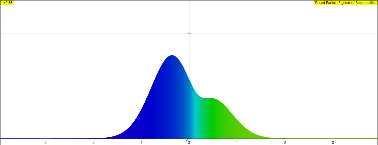
The Bound Energy Eigenstate Superposition JavaScript simulation allows users to visualize and explore the superposition principle by constructing time-dependent wave functions using the energy eigenfunctions of either an Infinite Square Well (ISW) or a Simple Harmonic Oscillator (SHO). Users can observe the evolution of wave functions formed by superposing different energy eigenstates and investigate concepts like wave packets and their motion.

What are some of the pre-set demonstrations and exercises available in the ISW part of the simulation?

The ISW part of the simulation includes pre-set demonstrations like "ISW Two State" (equal mix of ground and first excited states) and "ISW Gaussian" (various initial Gaussian wave packets). The exercises guide users to calculate energy levels and oscillation periods, observe the time evolution of superposition states, and analyze the behavior of Gaussian wave packets within the infinite square well.