About
Topics
KinematicsSpeed, velocity and acceleration
Graphical analysis of motion
Description
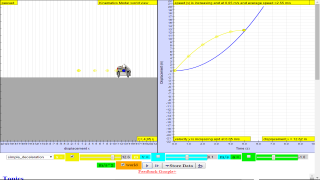
This simulation has a drop-down menu for exploration of(i) at rest use of progressive mathematical model is encouraged X = 0 for example
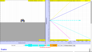
(ii) moving with uniform velocity, use of progressive mathematical model is encouraged for example X = 1*t for a constant velocity motion of v =1 m/s
(iii) moving with non-uniform velocity (eg, constant acceleration) use of progressive mathematical model is encouraged for example X = 0.5*1*t^2 for a constant acceleration motion of a =1 m/s^2
When only the velocity-time graph check-box is selected, it can be explored for the following cases too.
(i) at rest ,
(ii) moving with uniform velocity (eg, no acceleration)
(iii) moving with uniform acceleration (eg, constant acceleration = 9.81 m/s^2)
Sample Learning Goals
(f) deduce from the shape of a displacement-time graph when a body is:
(i) at rest example of progressive mathematical model is encouraged X = 0
(ii) moving with uniform velocity example of progressive mathematical model is encouraged X = 1*t for a constant velocity motion of v =1 m/s
(iii) moving with non-uniform velocity example of X = 0.5*1*t^2 for a constant acceleration motion of a =1 m/s^2
(g) deduce from the shape of a velocity-time graph when a body is:
(i) at rest
(ii) moving with uniform velocity
(iii) moving with uniform acceleration
(iv) moving with non-uniform acceleration
Version:
Translations
| Code | Language | Translator | Run | |
|---|---|---|---|---|
 |
||||
Credits
![]()
This email address is being protected from spambots. You need JavaScript enabled to view it.; tinatan
Creating a kinematics simulation of a moving car in 1D using JavaScript and HTML5 involves modeling the motion with parameters such as initial velocity, acceleration, time, and displacement. Below is a brief overview, study guide, and a sample code framework to implement such a simulation.
Document Brief:
Title: "Kinematics of a Moving Car in 1D: A Simulation with Tracker and Modeling"
This document describes the development of a 1D kinematics simulation for a car using JavaScript and HTML5. The applet allows users to input initial conditions (e.g., velocity, acceleration) and observe the car's motion. The simulation demonstrates fundamental kinematics concepts, providing both visual and data-driven outputs.
Study Guide:
Objective:
- To model and visualize the 1D motion of a car using kinematic equations.
- To explore the relationships between displacement, velocity, acceleration, and time.
Key Concepts:
-
Kinematic Equations:
- s=s0+v0t+12at2s = s_0 + v_0t + \frac{1}{2}at^2
- v=v0+atv = v_0 + at
- v2=v02+2a(s−s0)v^2 = v_0^2 + 2a(s - s_0)
-
Parameters:
- ss: Displacement
- v0v_0: Initial velocity
- aa: Acceleration
- tt: Time
-
1D Motion Assumptions:
- No friction or air resistance.
- Straight-line motion.
Sample Code Framework:
<!DOCTYPE html>
<html lang="en">
<head>
  <meta charset="UTF-8">
  <meta name="viewport" content="width=device-width, initial-scale=1.0">
  <title>1D Car Kinematics Simulation</title>
  <style>
    #simulationCanvas {
      border: 1px solid black;
      margin-top: 20px;
    }
    .controls {
      margin: 10px 0;
    }
  </style>
</head>
<body>
  <h1>1D Car Kinematics Simulation</h1>
  <div class="controls">
    <label>Initial Velocity (m/s): </label><input type="number" id="initialVelocity" value="5">
    <label>Acceleration (m/s²): </label><input type="number" id="acceleration" value="2">
    <label>Time Interval (s): </label><input type="number" id="timeInterval" value="0.1">
    <button onclick="startSimulation()">Start</button>
  </div>
  <canvas id="simulationCanvas" width="800" height="200"></canvas>

  <script>
    let canvas = document.getElementById('simulationCanvas');
    let ctx = canvas.getContext('2d');
    let carPosition = 50; // Initial position
    let time = 0;
    let animationFrame;

    function startSimulation() {
      const initialVelocity = parseFloat(document.getElementById('initialVelocity').value);
      const acceleration = parseFloat(document.getElementById('acceleration').value);
      const timeInterval = parseFloat(document.getElementById('timeInterval').value);

      carPosition = 50;
      time = 0;
      cancelAnimationFrame(animationFrame);

      function update() {
        time += timeInterval;
        carPosition = 50 + initialVelocity * time + 0.5 * acceleration * time * time;

        draw();
        animationFrame = requestAnimationFrame(update);
      }

      update();
    }

    function draw() {
      ctx.clearRect(0, 0, canvas.width, canvas.height);
      ctx.fillStyle = 'blue';
      ctx.fillRect(carPosition, canvas.height / 2 - 10, 50, 20); // Draw car
      ctx.font = '16px Arial';
      ctx.fillStyle = 'black';
      ctx.fillText(`Position: ${carPosition.toFixed(2)} m`, 10, 20);
    }
  </script>
</body>
</html>
App
 https://play.google.com/store/apps/details?id=com.ionicframework.kinematicstrackerapp897740
Topics
Kinematics
Speed, velocity and acceleration
Graphical analysis of motion
Description
This simulation has a drop-down menu for exploration of
(i) at rest use of progressive mathematical model is encouraged X = 0 for example
(ii) moving with uniform velocity, use of progressive mathematical model is encouraged for example X = 1*t for a constant velocity motion of v =1 m/s
(iii) moving with non-uniform velocity (eg, constant acceleration) use of progressive mathematical model is encouraged for example X = 0.5*1*t^2 for a constant acceleration motion of a =1 m/s^2
When only the velocity-time graph check-box is selected, it can be explored for the following cases too.
(i) at rest ,
(ii) moving with uniform velocity (eg, no acceleration)
(iii) moving with uniform acceleration (eg, constant acceleration = 9.81 m/s^2)
(iv) moving with non-uniform acceleration
Sample Learning Goals
(e) plot and interpret a displacement-time graph and a velocity-time graph
(f) deduce from the shape of a displacement-time graph when a body is:
(i) at rest example of progressive mathematical model is encouraged X = 0
(ii) moving with uniform velocity example of progressive mathematical model is encouraged X = 1*tfor a constant velocity motion of v =1 m/s
(iii) moving with non-uniform velocity example of X = 0.5*1*t^2 for a constant acceleration motion of a =1 m/s^2
(g) deduce from the shape of a velocity-time graph when a body is:
(i) at rest
(ii) moving with uniform velocity
(iii) moving with uniform acceleration
(iv) moving with non-uniform acceleration
Worksheet
- Slides for Workshop Link1 , Link2
- Final version Link1, Link2 by Lyna, Gavin, Dave and lookang
- Motion in One Dimension student worksheet (dl-gwf) Link1, Link2 by Lyna, Gavin, Dave and lookang
Video
- https://youtu.be/ZYIeBKDBXU8 Kinematics 1d simulation video tutorial with modeling pedagogy by lookang lawrence wee
- https://youtu.be/SsSPd6I4BnA Kinematics 1D simulation running on hmtl5 Modeling pedagogy 2 by lookang lawrence wee
- Kinematics Simulation - Secondary & JC by Dave Lommen
Pedagogical Writeup
| Process | Lesson Implementation | |
| Sub-Process(es) | Introducing the Lesson / Arousing and Sustaining Interest | |
| Teaching Action | Mystery | |
Technology:
Mystery could take the form of to describe it in an equation, called model.
Give the challenge to solve the mystery of a predictive equation that can be use to tell the future, more precisely the movement of a car, in a physics lesson.
Through the model selected by the students, it gives an indication of the students prior knowledge about what they know now, so that the teacher can understand the gaps of understanding for personalised mentoring
| Process | Lesson Implementation | |
| Sub-Process(es) | Introducing the Lesson / Arousing and Sustaining Interest | |
| Teaching Action | Little Professor/Little Teachers | |
Technology:
use exisiting schools' learning management system such as https://www.edmodo.com/ or Whatapp group chat to allow of arousing and sustaining interest.
Other simulations
- http://www.physicsclassroom.com/Physics-Interactives/1-D-Kinematics/Graphs-and-Ramps
- http://www.thephysicsaviary.com/Physics/Programs/Labs/EquationsOfMotionLab/index.html
- https://www.geogebra.org/m/gagswmru by h
Project related:
Understanding Teacher Learning Community as Support for Implementation of Open Source Physics for Conceptual Instruction
Project Number: OER 10/15 GWF
Project Duration: 01 July 2015 - 30 April 2017
http://weelookang.blogspot.sg/2015/07/understanding-teacher-learning.html
Family of Resources
| Secondary | Primary | ||||||||||||||||||||
About
TopicsKinematicsSpeed, velocity and acceleration Graphical analysis of motion DescriptionThis simulation has a drop-down menu for exploration of(i) at rest use of progressive mathematical model is encouraged X = 0 for example (ii) moving with uniform velocity, use of progressive mathematical model is encouraged for example X = 1*t for a constant velocity motion of v =1 m/s (iii) moving with non-uniform velocity (eg, constant acceleration) use of progressive mathematical model is encouraged for example X = 0.5*1*t^2 for a constant acceleration motion of a =1 m/s^2 When only the velocity-time graph check-box is selected, it can be explored for the following cases too. (i) at rest , (ii) moving with uniform velocity (eg, no acceleration) (iii) moving with uniform acceleration (eg, constant acceleration = 9.81 m/s^2) Sample Learning Goals
(e) plot and interpret a displacement-time graph and a velocity-time
graph
(f) deduce from the shape of a displacement-time graph when a body is: (i) at rest example of progressive mathematical model is encouraged X = 0 (ii) moving with uniform velocity example of progressive mathematical model is encouraged X = 1*t for a constant velocity motion of v =1 m/s (iii) moving with non-uniform velocity example of X = 0.5*1*t^2 for a constant acceleration motion of a =1 m/s^2 (g) deduce from the shape of a velocity-time graph when a body is: (i) at rest (ii) moving with uniform velocity (iii) moving with uniform acceleration (iv) moving with non-uniform acceleration Version:Translations
Credits
|
||||||||||||||||||||
FAQ:
-
What concepts does this simulation demonstrate?
- It demonstrates the principles of 1D motion using kinematic equations and visually represents the displacement over time.
-
How can this be extended to 2D motion?
- By adding horizontal and vertical components of velocity and acceleration, extending the equations to include both dimensions.
-
What inputs are required?
- Initial velocity, acceleration, and optionally, the time interval for numerical updates.
-
How does this relate to Tracker?
- The simulation models similar scenarios analyzed with Tracker software, providing insights into how physical quantities evolve during motion.
-
What are the practical applications?
- Education, visualization of vehicle dynamics, and introductory physics simulations.
- Details
- Parent Category: 03 Motion & Forces
- Category: 01 Kinematics
- Hits: 12674


