PICUP EXERCISE 2: IRRADIANCE DUE TO N N POINT SOURCES WITH A RECTANGULAR APERTURE has bug JavaScript Model Simulation Virtual Lab

Breadcrumbs

About

Intro Page

Shadows (Ray Optics)

Developed by E. Behringer

This set of exercises guides the student in exploring computationally the behavior of light patterns and shadows generated by simple light sources together with apertures in thin, opaque barriers. It requires the student to generate, and describe the results of simulating, light patterns and shadows. Diffraction is ignored. The numerical approach used is summing over a two-dimensional spatial grid while applying a logical mask (‘transparency function’). Please note that this set of computational exercises can be affordably coupled to simple experiments with small light bulbs and apertures cut into (or barriers cut out of) opaque paper sheets. A possible extension is to compare the predicted light patterns to experimental measurements. This set of exercises could be incorporated as an initial activity in an intermediate optics laboratory.

Subject Area	Waves & Optics
Levels	First Year and Beyond the First Year
Available Implementation	Python
Learning Objectives	Students who complete this set of exercises will be able to predict and visually represent the irradiance distribution at a screen generated by a point light source and an aperture (Exercise 1); predict and visually represent the irradiance distribution at a screen generated by multiple point light sources and an aperture (Exercise 2); predict and visually represent the irradiance distribution at a screen generated by multiple point light sources and a complex aperture (Exercise 3); predict and visually represent the irradiance distribution at a screen generated by a two-dimensional array of point light sources and an aperture (Exercise 4);, and predict and visually represent the irradiance distribution at a screen generated by a two-dimensional array of point light sources and an opaque barrier (Exercise 5).
Time to Complete	120 min

Shadows_Exercise_2.py

# Shadows_Exercise_2.py

# A linear array of N point sources located a specified distance from

# a rectangular aperture that is centered on the origin.

# A screen is located a specified distance from

# the aperture.

# This file will generate a filled contour plot of

# the irradiance of light reaching the screen

# versus lateral coordinates (x,y)

# Written by:

# Ernest R. Behringer

# Department of Physics and Astronomy

# Eastern Michigan University

# Ypsilanti, MI 48197

# (734) 487-8799

# ebehringe@emich.edu

# 20160112-13 original code by ERB

# 20160609 clean up by ERB

# import the commands needed to make the plot

from pylab import xlabel,ylabel,xlim,ylim,axis,show,contourf,colorbar,figure,title

from matplotlib import cm

# import the command needed to make a 1D array

from numpy import meshgrid,absolute,where,zeros,linspace

# inputs

zs = -20.0 # distance between the source and aperture [cm]

zsc = 40.0 # distance between the screen and aperture [cm]

nso = 3 # number of point sources

length_so = 4.0 # length of the array of point sources [cm]

ap_width = 4.0 # aperture width [cm]

ap_height = 3.0 # aperture height [cm]

screen_width = 60.0 # screen width [cm]

screen_height = 60.0 # wcreen height [cm]

nw = 240 # Number of screen width intervals

nh = 240 # Number of screen height intervals

# initialize needed arrays to zero

rso = zeros((nso,2)) # (x,y) source positions [cm,cm]

screen_x = zeros((nw+1,nh+1)) # x-coordinates of screen points

screen_y = zeros((nw+1,nh+1)) # y-coordinates of screen points

rsq = zeros((nw+1,nh+1)) # r squared values

irradiance = zeros((nw+1,nh+1)) # irradiance values

x0 = zeros((nw+1,nh+1)) # x-coordinates of intersections at aperture plane

y0 = zeros((nw+1,nh+1)) # y-coordinates of intersections at aperture plane

# create 1D arrays to create a meshgrid for contour plotting

screen_xx = linspace(-0.5*screen_width,0.5*screen_width,nw+1)

screen_yy = linspace(-0.5*screen_height,0.5*screen_height,nh+1)

# generate the meshgrid of screen points

screen_xx, screen_yy = meshgrid(screen_xx,screen_yy)

# Set up point source coordinates

# Here, the sources are arranged

for i in range (0,nso):

for j in range (0,2):

if j==0:

rso[i,j] = -0.5*length_so + i*length_so/(nso-1)

else: # j = 1 and the y-coordinate is

rso[i,j] = 0.0

# Calculate grid increments

deltaw = screen_width/nw # grid increment, width [cm]

deltah = screen_height/nh # grid increment, height [cm]

# Define the array of screen x and screen y values

for i in range (0,nw+1):

for j in range (0,nh+1):

screen_x[i,j] = -0.5*screen_width + deltaw*i

screen_y[i,j] = -0.5*screen_height + deltah*j

# Calculate the irradiance at each screen point

for k in range (0,nso):

for i in range (0,nw+1):

for j in range (0,nh+1):

# First calculate square of distance from source to screen

rsq = (screen_x[i,j]-rso[k,0])**2 + (screen_y[i,j]-rso[k,1])**2 + (zsc - zs)**2

# Calculate x and y coordinates at the aperture

x0[i,j] = rso[k,0] + abs(zs)*(screen_x[i,j] - rso[k,0])/(zsc - zs)

y0[i,j] = rso[k,1] + abs(zs)*(screen_y[i,j] - rso[k,1])/(zsc - zs)

# Check if the coordinates fall within the aperture

maskx = where(absolute(x0) < 0.5*ap_width,1.0,0.0)

masky = where(absolute(y0) < 0.5*ap_height,1.0,0.0)

# Calculate the irradiance (note that we are accumulating irradiance)

irradiance = irradiance + maskx*masky/rsq

# make a filled contour plot of the period vs overlap and length ratios

figure()

contourf(screen_yy,screen_xx,irradiance,100,cmap=cm.bone)

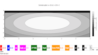
title('Illumination pattern: $w =$ %s cm, $h =$ %s; $N =$ %d'%(ap_width,ap_height,nso))

axis('equal')

xlim(-0.5*screen_width,0.5*screen_width)

ylim(-0.5*screen_height,0.5*screen_height)

xlabel(" $x$ [cm]")

ylabel(" $y$ [cm]")

colorbar().set_label(label='Irradiance [arb. units]',size=16)

show()

Exercise 2

EXERCISE 2: IRRADIANCE DUE TO POINT SOURCES WITH A RECTANGULAR APERTURE

If instead of one point source, suppose point sources are uniformly spaced and also arranged along a line segment of total length that is parallel to the -axis, as shown below.

Calculate the irradiance at the screen for the aperture of Exercise 1 if one source is on the symmetry axis, cm, and: (a) ; (b) ; (c) and . How many distinct shadow regions (areas characterized by different irradiance) appear in each case?

Translations

Code	Language		Translator	Run

Credits

Fremont Teng; Loo Kang Wee; based on codes by E. Behringer

1. Overview and Context:

The material presents a computational exercise (Exercise 2 within a larger set) designed to help students understand the behavior of light patterns and shadows created by multiple point light sources passing through a rectangular aperture. This exercise builds upon a previous one (Exercise 1) that likely dealt with a single point source. Diffraction is explicitly ignored in this model, focusing on ray optics principles and a numerical summation approach.

The broader context is a series of computational physics exercises ("PICUP") intended for first-year undergraduate physics students and beyond. These exercises aim to bridge computational modeling with potential hands-on experiments using simple light sources and apertures. The platform utilizes EasyJavaScriptSimulation for interactive models and also provides Python code examples for the simulations.

2. Core Learning Objective of Exercise 2:

The primary learning objective of Exercise 2 is for students to be able to:

"predict and visually represent the irradiance distribution at a screen generated by multiple point light sources and an aperture."

This involves understanding how the superposition of light from multiple sources, after passing through an aperture, affects the intensity (irradiance) pattern observed on a screen.

3. Simulation Methodology:

The simulation employs a numerical approach based on:

Summing over a two-dimensional spatial grid: The screen is discretized into a grid of points.
Applying a logical mask (‘transparency function’): The rectangular aperture acts as a mask, only allowing light rays passing through it to reach the screen.
Ray Optics: Diffraction effects are not considered; light travels in straight lines from the sources, through the aperture, to the screen.

4. Python Code Implementation (Shadows_Exercise_2.py):

The provided Python code snippet illustrates how the simulation for Exercise 2 is implemented. Key aspects of the code include:

Defining Inputs: The code sets various parameters such as:
zs: distance between the source and aperture.
zsc: distance between the screen and aperture.
nso: number of point sources.
length_so: length of the array of point sources.
ap_width: aperture width.
ap_height: aperture height.
screen_width, screen_height: dimensions of the screen.
nw, nh: number of grid intervals on the screen.
Initializing Arrays: NumPy arrays are initialized to store source positions (rso), screen coordinates (screen_x, screen_y), squared distances (rsq), irradiance values (irradiance), and intersection points at the aperture plane (x0, y0).
Setting up Source Coordinates: The code explicitly arranges the nso point sources in a linear array along the x-axis, centered around y=0, with a total length length_so.
for i in range (0,nso):
for j in range (0,2):
if j==0:
rso[i,j] = -0.5*length_so + i*length_so/(nso-1)
else: # j = 1 and the y-coordinate is
rso[i,j] = 0.0
Calculating Irradiance: The core of the simulation involves nested loops iterating through each point source and each point on the screen. For each source-screen point pair:
The squared distance between the source and screen is calculated.
The coordinates (x0, y0) where the line from the source to the screen intersects the aperture plane are determined using similar triangles based on the distances.
A "mask" (maskx, masky) is applied to check if these intersection coordinates fall within the dimensions of the rectangular aperture. The mask is 1.0 if the intersection is within the aperture and 0.0 otherwise.
The irradiance at the screen point due to the current source is calculated as maskx*masky/rsq (inversely proportional to the square of the distance) and accumulated in the irradiance array.
Generating a Contour Plot: Finally, the code uses matplotlib.pyplot to generate a filled contour plot of the calculated irradiance distribution on the screen. The plot includes a title indicating the aperture dimensions and the number of sources.

5. Exercise Questions:

Exercise 2 poses specific questions for the students to investigate:

Using the aperture dimensions from Exercise 1.
With one source on the symmetry axis and a total source length L = 4.0 cm.
Students are asked to calculate the irradiance for three different numbers of point sources: (a) N = 3, (b) N = 11, and (c) N = 101.
The key question is: "How many distinct shadow regions (areas characterized by different irradiance) appear in each case?" This prompts students to analyze the resulting irradiance patterns and relate them to the number and arrangement of the light sources.

6. Pedagogical Implications:

This exercise provides a hands-on (or rather, computationally-driven) approach to understanding:

The principle of superposition of light intensity.
How the spatial distribution of light sources affects the resulting shadow patterns after passing through an aperture.
The transition from a discrete number of sources to a more continuous light source as the number of point sources increases.
The relationship between ray optics and the formation of shadows.

The suggestion to couple this with simple physical experiments reinforces the connection between computational models and real-world phenomena.

7. Noteworthy Points:

The exercise explicitly ignores diffraction, simplifying the model to geometric optics.
The use of Python and the availability of a JavaScript simulation make this exercise accessible to students with varying levels of computational skills.
The focus on "distinct shadow regions" encourages qualitative analysis of the simulation results in addition to the quantitative irradiance data.

In conclusion, "PICUP EXERCISE 2" is a valuable learning activity that utilizes computational modeling to explore the concept of irradiance distribution from multiple point sources passing through a rectangular aperture. It encourages students to predict, visualize, and analyze the resulting light patterns, fostering a deeper understanding of basic optical principles.

Study Guide: Irradiance Due to Multiple Point Sources and a Rectangular Aperture

Overview

This study guide focuses on the concepts and computational approach presented in the PICUP Exercise 2, which explores the irradiance pattern generated on a screen by multiple point light sources passing through a rectangular aperture. The exercise utilizes a numerical simulation method, ignoring diffraction effects, to predict and visualize these patterns. Understanding this exercise involves grasping the geometry of the setup, the principle of superposition of light (implicitly), and the application of a transparency function defined by the aperture.

Key Concepts

Irradiance: The power of electromagnetic radiation incident per unit area on a surface. In this context, it refers to the intensity of light reaching the screen.
Point Source: A source of light that emits radiation from a single, infinitesimally small point in space. While not physically realistic, it serves as a useful idealization.
Aperture: An opening or hole in an opaque barrier that allows light to pass through. In this exercise, the aperture is rectangular.
Transparency Function: A mathematical function that describes which parts of a plane are transparent (allow light to pass) and which are opaque (block light). For the rectangular aperture, this function acts as a logical mask.
Superposition: The principle that the total irradiance at a point on the screen due to multiple light sources is the sum of the irradiances produced by each source individually (although this exercise calculates it iteratively).
Ray Optics: An approximation of light propagation that treats light as traveling in straight lines (rays), neglecting wave phenomena like diffraction. This is the underlying assumption of this exercise.
Computational Simulation: Using numerical methods and computer code to model a physical system and predict its behavior. This exercise uses Python and libraries like NumPy and Matplotlib.
Spatial Grid: A two-dimensional array of points used to represent the screen and the aperture plane in the numerical simulation.
Contour Plot: A graphical representation of a function of two variables as level curves of constant value, often used here to visualize the irradiance distribution.

Quiz

Describe the physical setup modeled in PICUP Exercise 2. What are the key components and their relative positions?
What is the purpose of the 'transparency function' in the simulation, and how is it implemented for a rectangular aperture?
How does the simulation calculate the irradiance at a single point on the screen due to one of the point sources? What factors are considered?
Explain how the simulation accounts for multiple point sources to determine the total irradiance at the screen. What principle is implicitly used?
What are the learning objectives of this exercise, as stated in the "About" section of the resource?
What programming language is used for the provided code (Shadows_Exercise_2.py), and what are some of the imported libraries and their general functions?
In the provided Python code, what do the variables zs, zsc, and rso represent?
Explain the role of the meshgrid function in the Python code. What variables are created using it, and what do they represent?
How are the coordinates of the intersection points at the aperture plane (x0, y0) calculated in the code? What geometric principle is being applied?
What does the contourf function from matplotlib.pyplot do in the provided Python code, and what does the resulting plot represent?

Quiz Answer Key

The setup consists of a linear array of N point light sources located at a specified distance (zs) from a rectangular aperture. A screen is placed at another specified distance (zsc) from the aperture. The simulation calculates the irradiance pattern on this screen.
The transparency function acts as a mask to determine whether light rays passing through a particular point in the aperture plane reach the screen. For a rectangular aperture, it checks if the x and y coordinates at the aperture fall within the defined width and height, assigning a value of 1 (transparent) if they do, and 0 (opaque) otherwise.
For a single point source, the simulation calculates the squared distance (rsq) from the source to each point on the screen. The irradiance is then proportional to the transparency of the corresponding point in the aperture divided by this squared distance.
The simulation calculates the irradiance at each screen point due to each individual point source and then sums these contributions. This implicitly uses the principle of superposition, assuming the intensities of the light sources add linearly.
The learning objectives include the ability to predict and visually represent the irradiance distribution at a screen generated by a point light source and an aperture, multiple point light sources and an aperture, multiple point light sources and a complex aperture, a two-dimensional array of point light sources and an aperture, and a two-dimensional array of point light sources and an opaque barrier (though Exercise 2 specifically focuses on the second objective).
The programming language is Python. The imported libraries include pylab (which includes matplotlib.pyplot for plotting) for creating the contour plot, labels, and colorbar, and numpy for creating and manipulating numerical arrays like meshgrid, zeros, linspace, and where.
zs represents the distance between the source(s) and the aperture [cm]. zsc represents the distance between the screen and the aperture [cm]. rso is a NumPy array storing the (x, y) coordinates of each of the N point sources [cm, cm].
The meshgrid function takes two 1D arrays (screen_xx and screen_yy) and returns two 2D coordinate matrices (screen_xx, screen_yy). These matrices represent all the x and y coordinates of the points on the screen, forming the spatial grid on which the irradiance is calculated and plotted.
The coordinates at the aperture plane (x0[i,j], y0[i,j]) are calculated using similar triangles formed by the source, the aperture, and the screen. The formulas effectively project the line from the source through a screen point back to the aperture plane based on the distances zs and zsc.
The contourf function creates a filled contour plot. In this code, it takes the y-coordinates, x-coordinates of the screen points, and the calculated irradiance values as input to generate a visual representation of the irradiance distribution on the screen, with different colors representing different irradiance levels.

Essay Format Questions

Discuss the limitations of the ray optics approximation used in this exercise, particularly when considering real-world light sources and apertures. How might diffraction phenomena alter the observed irradiance patterns?
Explain the relationship between the number and spacing of the point sources in the linear array and the resulting irradiance pattern on the screen after passing through the rectangular aperture. Consider cases with few and many sources.
Describe how the dimensions and position of the rectangular aperture influence the shape and intensity of the irradiance pattern observed on the screen when illuminated by multiple point sources.
The exercise mentions the possibility of coupling the computational simulations with simple experiments. Outline a possible experimental setup using basic materials and discuss how the predicted light patterns could be compared to experimental measurements. What challenges might arise in such a comparison?
Analyze the structure and logic of the provided Python code (Shadows_Exercise_2.py). Explain how the code implements the physical model described in the exercise, highlighting the key steps in the calculation of the irradiance distribution.

Glossary of Key Terms

Irradiance: The power per unit area received by a surface in the form of electromagnetic radiation. Often referred to as intensity.
Point Source: An idealized light source that emits light from a single point in space.
Aperture: An opening or hole that allows light to pass through an otherwise opaque barrier.
Transparency Function: A mathematical description of how much light is transmitted through different parts of a surface or plane.
Ray Optics: A model of light propagation where light travels in straight lines called rays, neglecting wave effects.
Computational Simulation: The use of computer programs to model the behavior of a physical system over time or under different conditions.
Spatial Grid: A discrete representation of a continuous space using a network of points or cells.
Contour Plot: A graphical technique for representing a 3D surface by plotting constant elevation curves (isobars, isotherms, etc.) on a 2D map. In this case, it represents constant irradiance.
Superposition: The principle that the net effect at a given point is the sum of the individual effects. In optics (ignoring interference in this ray optics model), the total irradiance is the sum of irradiances from individual sources.
Logical Mask: A function or array that selects or filters data based on a logical condition (e.g., inside or outside the aperture).

Version:

Frequently Asked Questions: Irradiance from Multiple Point Sources through a Rectangular Aperture

1. What is the purpose of this computational exercise? This exercise aims to help students understand and visualize the light patterns and shadows created when light from multiple point sources passes through a rectangular aperture and falls on a screen. Students are expected to computationally generate and analyze these irradiance distributions.

2. What physical phenomena are being explored in this exercise? The primary physical phenomenon explored is the superposition of light from multiple point sources after passing through an aperture. The exercise focuses on ray optics and geometrically determined shadows and light patterns, explicitly ignoring diffraction effects.

3. How is the irradiance distribution calculated in the simulation? The simulation calculates the irradiance at the screen by summing the contributions from each point source. For each point source and each point on the screen, it determines if the light ray passing through the aperture would reach that screen point. This is done by applying a logical mask based on the aperture's dimensions. The irradiance contribution from each source is inversely proportional to the square of the distance from the source to the screen.

4. What parameters can be varied in this simulation? Based on the provided code and exercise description, several parameters can be varied, including:

The number of point sources (nso).
The distance between the source(s) and the aperture (zs).
The distance between the screen and the aperture (zsc).
The total length of the array of point sources (length_so).
The width (ap_width) and height (ap_height) of the rectangular aperture.
The width (screen_width) and height (screen_height) of the screen.
The number of intervals used to discretize the screen width (nw) and height (nh), affecting the resolution of the simulation.

5. What is the role of the rectangular aperture in shaping the irradiance pattern? The rectangular aperture acts as a spatial filter, allowing only the light rays that pass through its opening to reach the screen. It casts a geometric shadow corresponding to its shape, and with multiple light sources, the superposition of these individual shadows creates a more complex irradiance distribution with regions of varying intensity.

6. How does increasing the number of point sources affect the irradiance pattern on the screen? Increasing the number of point sources, while keeping the total length of the source array constant, leads to a more complex irradiance pattern on the screen. Instead of a single well-defined shadow (as with a single point source), multiple overlapping shadows from each source passing through the aperture are generated. This results in regions with varying degrees of illumination, from fully illuminated areas to regions blocked by shadows from multiple sources. As the number of sources increases and become more closely spaced, the pattern may begin to resemble the pattern created by a continuous light source of the same size.

7. What does the filled contour plot of irradiance represent? The filled contour plot visually represents the irradiance distribution on the screen. Different colors or shades on the plot correspond to different levels of irradiance. The x and y axes of the plot represent the lateral coordinates on the screen, allowing students to see how the intensity of light varies across the screen's surface. The colorbar provides a key to interpret the irradiance values.

8. What is the significance of ignoring diffraction in this exercise? By ignoring diffraction, this exercise focuses on the principles of ray optics and the formation of geometric shadows. Diffraction effects, which cause light to bend around obstacles and spread out after passing through an aperture, are not considered. This simplification allows students to first grasp the basic concepts of shadow formation and superposition with multiple light sources based purely on the paths of light rays. Diffraction would introduce more complex patterns, such as fringes at the edges of shadows.

1 1 1 1 1 1 1 1 1 1 Rating 0.00 (0 Votes)

Details: Written by Loo Kang Wee; Parent Category: 03 Waves; Category: 04 Light; Published: 15 April 2016; Created: 15 April 2016; Last Updated: 22 March 2025; Hits: 6275