PICUP EXERCISE 3: IRRADIANCE DUE TO N N POINT SOURCES AND AN L-SHAPED APERTURE has bug JavaScript Model Simulation Virtual Lab

Breadcrumbs

About

Intro Page

Shadows (Ray Optics)

Developed by E. Behringer

This set of exercises guides the student in exploring computationally the behavior of light patterns and shadows generated by simple light sources together with apertures in thin, opaque barriers. It requires the student to generate, and describe the results of simulating, light patterns and shadows. Diffraction is ignored. The numerical approach used is summing over a two-dimensional spatial grid while applying a logical mask (‘transparency function’). Please note that this set of computational exercises can be affordably coupled to simple experiments with small light bulbs and apertures cut into (or barriers cut out of) opaque paper sheets. A possible extension is to compare the predicted light patterns to experimental measurements. This set of exercises could be incorporated as an initial activity in an intermediate optics laboratory.

Subject Area	Waves & Optics
Levels	First Year and Beyond the First Year
Available Implementation	Python
Learning Objectives	Students who complete this set of exercises will be able to predict and visually represent the irradiance distribution at a screen generated by a point light source and an aperture (Exercise 1); predict and visually represent the irradiance distribution at a screen generated by multiple point light sources and an aperture (Exercise 2); predict and visually represent the irradiance distribution at a screen generated by multiple point light sources and a complex aperture (Exercise 3); predict and visually represent the irradiance distribution at a screen generated by a two-dimensional array of point light sources and an aperture (Exercise 4);, and predict and visually represent the irradiance distribution at a screen generated by a two-dimensional array of point light sources and an opaque barrier (Exercise 5).
Time to Complete	120 min

Exercise 3

EXERCISE 3: IRRADIANCE DUE TO POINT SOURCES AND AN L-SHAPED APERTURE

Now imagine that you have point sources, as in Exercise 2, but now the aperture is an L-shaped aperture as shown below.

What do you expect the irradiance pattern at the screen to look like? Why? Now calculate the irradiance pattern at the screen for the case and cm. Does the computed pattern resemble your prediction?

Shadows_Exercise_3.py

# Shadows_Exercise_3.py

# A linear array of N point sources located a specified distance from

# an L-shaped aperture composed of two rectangular apertures,

# one of which is centered on the origin.

# A screen is located a specified distance from

# the aperture.

# This file will generate a filled contour plot of

# the irradiance of light reaching the screen

# versus lateral coordinates (x,y)

# Written by:

# Ernest R. Behringer

# Department of Physics and Astronomy

# Eastern Michigan University

# Ypsilanti, MI 48197

# (734) 487-8799

# ebehringe@emich.edu

# 20160112-13 by ERB one aperture

# 20160119 by ERB compound aperture

# 20160609 clean up by ERB

# import the commands needed to make the plot

from pylab import axis,xlim,ylim,xlabel,ylabel,show,contourf,colorbar,figure,title

from matplotlib import cm

# import the command needed to make a 1D array

from numpy import meshgrid,absolute,where,zeros,linspace

# inputs

zs = -20.0 # distance between the source and aperture [cm]

zsc = 40.0 # distance between the screen and aperture [cm]

nso = 101 # number of point sources

length_so = 4.0 # length of the array of point sources [cm]

ap1_width = 2.0 # aperture width [cm]

ap1_height = 1.0 # aperture height [cm]

ap2_width = 1.0 # second aperture width [cm]

ap2_height = 3.0 # second aperture height [cm]

ap2_x = -0.5 # second aperture center x-coordinate [cm]

ap2_y = 2.0 # second aperture center y coordinate [cm]

screen_width = 60.0 # screen width [cm]

screen_height = 60.0 # wcreen height [cm]

nw = 240 # Number of screen width intervals

nh = 240 # Number of screen height intervals

# initialize needed arrays to zero

rso = zeros((nso,2)) # (x,y) location of the source [cm,cm]

screen_x = zeros((nw+1,nh+1)) # x-coordinates of screen points

screen_y = zeros((nw+1,nh+1)) # y coordinates of screen points

rsq = zeros((nw+1,nh+1)) # r squared values

irradiance = zeros((nw+1,nh+1)) # irradiance values

x0 = zeros((nw+1,nh+1)) # x coordinate of intersection at aperture plane

y0 = zeros((nw+1,nh+1)) # y coordinate of intersection at aperture plane

# create 1D arrays to create a meshgrid for contour plotting

screen_xx = linspace(-0.5*screen_width,0.5*screen_width,nw+1)

screen_yy = linspace(-0.5*screen_height,0.5*screen_height,nh+1)

# generate the meshgrid

screen_xx, screen_yy = meshgrid(screen_xx,screen_yy)

# Set up point source coordinates

for i in range (0,nso):

for j in range (0,2):

if j==0: # the x-coordinate is

rso[i,j] = -0.5*length_so + i*length_so/(nso-1)

else: # j = 1 and the y-coordinate is

rso[i,j] = 0.0

# Calculate grid increments

deltaw = screen_width/nw # grid increment, width [cm]

deltah = screen_height/nh # grid increment, height [cm]

# Define the array of screen x and screen y values

for i in range (0,nw+1):

for j in range (0,nh+1):

screen_x[i,j] = -0.5*screen_width + deltaw*i

screen_y[i,j] = -0.5*screen_height + deltah*j

# Calculate the irradiance at each screen point

for k in range (0,nso):

for i in range (0,nw+1):

for j in range (0,nh+1):

# First calculate square of distance from source to screen

rsq[i,j] = (screen_x[i,j]-rso[k,0])**2 + (screen_y[i,j]-rso[k,1])**2 + (zsc-zs)**2

# Calculate x and y coordinates at the aperture

x0[i,j] = rso[k,0] + abs(zs)*(screen_x[i,j] - rso[k,0])/(zsc - zs)

y0[i,j] = rso[k,1] + abs(zs)*(screen_y[i,j] - rso[k,1])/(zsc - zs)

# Check if the ray coordinates at the aperture fall within the apertures

maskx1 = where(absolute(x0) < 0.5*ap1_width,1.0,0.0)

masky1 = where(absolute(y0) < 0.5*ap1_height,1.0,0.0)

maskx2 = where((x0 < ap2_x + 0.5*ap2_width)&(x0 > ap2_x - 0.5*ap2_width),1.0,0.0)

masky2 = where((y0 < ap2_y + 0.5*ap2_height)&(y0 > ap2_y - 0.5*ap2_height),1.0,0.0)

# Calculate the irradiance (note that we are accumulating irradiance)

irradiance = irradiance + (maskx1*masky1 + maskx2*masky2)/rsq

# make a filled contour plot of the period vs overlap and length ratios

figure()

contourf(screen_yy,screen_xx,irradiance,100,cmap=cm.bone)

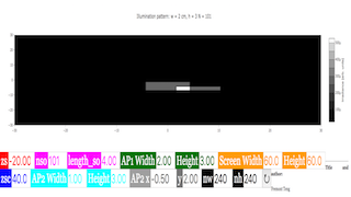
title('Illumination pattern: $w =$ %s cm, $h =$ %s; $N =$ %d'%(ap1_width,ap1_height,nso))

axis('equal')

xlim(-0.5*screen_width,0.5*screen_width)

ylim(-0.5*screen_height,0.5*screen_height)

xlabel(" $x$ [cm]")

ylabel(" $y$ [cm]")

colorbar().set_label(label='Irradiance [arb. units]',size=16)

show()

Translations

Code	Language		Translator	Run

Credits

Fremont Teng; Loo Kang Wee

Overview:

This document provides a briefing on "PICUP Exercise 3," a computational physics exercise focused on understanding the irradiance distribution produced by multiple point light sources passing through an L-shaped aperture and projected onto a screen. This exercise is part of a larger set designed to computationally explore light patterns and shadows using ray optics, ignoring diffraction effects. The exercise utilizes a numerical approach involving summing over a two-dimensional spatial grid and applying a transparency function (the aperture).

Main Themes and Important Ideas:

Computational Exploration of Light Patterns and Shadows: The core theme of this exercise is to use computational simulation to predict and visualize light patterns and shadows. The "About" section explicitly states: "This set of exercises guides the student in exploring computationally the behavior of light patterns and shadows generated by simple light sources together with apertures in thin, opaque barriers. It requires the student to generate, and describe the results of simulating, light patterns and shadows."
Multiple Point Sources: Building upon previous exercises (mentioned as "Exercise 2"), this exercise introduces the concept of irradiance from multiple (N) point light sources. The exercise prompts the user to consider the combined effect of these sources on the resulting light pattern.
Complex Aperture Shape: The key distinguishing feature of Exercise 3 is the introduction of a more complex aperture – an "L-shaped aperture" composed of two rectangular apertures. This challenges the user to think about how the shape of the aperture influences the final irradiance distribution. The description states, "Now imagine that you have N N point sources, as in Exercise 2, but now the aperture is an L-shaped aperture as shown below."
Ray Optics Approximation: The exercise operates under the principles of ray optics, explicitly stating that "Diffraction is ignored." This simplification allows for a geometrical approach to determining which light rays pass through the aperture and reach the screen.
Irradiance Distribution: The primary goal is to "predict and visually represent the irradiance distribution at a screen." The exercise involves calculating and then visualizing the intensity of light at different points on the screen after passing through the aperture. The associated Python script aims to generate a "filled contour plot of the irradiance of light reaching the screen versus lateral coordinates (x,y)."
Numerical Simulation using a Spatial Grid: The "About" section mentions the numerical method: "The numerical approach used is summing over a two-dimensional spatial grid while applying a logical mask (‘transparency function’)." This indicates that the simulation works by dividing the space into discrete points and determining if light from each source reaches each screen point through the open areas of the aperture.
Practical Connection to Experiments: The description encourages linking the computational exercises to real-world experiments: "Please note that this set of computational exercises can be affordably coupled to simple experiments with small light bulbs and apertures cut into (or barriers cut out of) opaque paper sheets. A possible extension is to compare the predicted light patterns to experimental measurements." This highlights the pedagogical value of connecting theoretical simulations with observable phenomena.
Learning Objectives: Exercise 3 specifically aims to enable students to "predict and visually represent the irradiance distribution at a screen generated by multiple point light sources and a complex aperture." This clearly defines the intended learning outcome.
Specific Simulation Parameters: The exercise provides specific parameters for simulation, such as "N = 101" point sources and an aperture width "w = 2.0 cm." It then asks, "Does the computed pattern resemble your prediction?" This encourages students to form a hypothesis before running the simulation and then compare their prediction with the computational result.
Python Implementation: The provided "Shadows_Exercise_3.py" script indicates that the simulation is implemented in Python using libraries like pylab and numpy for plotting and numerical calculations. The script defines the setup, including source and screen distances, aperture dimensions, and the numerical grid. It then calculates the irradiance by summing contributions from each point source that pass through the aperture.

Key Facts from the Source:

Exercise Focus: Investigating irradiance patterns from N point sources through an L-shaped aperture.
Underlying Physics: Ray optics, ignoring diffraction.
Methodology: Numerical simulation on a 2D spatial grid using a transparency function for the aperture.
Software: Implemented in Python using pylab and numpy.
Simulation Parameters: Example parameters given are N = 101 point sources and an aperture width of 2.0 cm. The script also defines other geometrical parameters like source-aperture distance (zs = -20.0 cm), aperture-screen distance (zsc = 40.0 cm), aperture dimensions (ap1_width, ap1_height, ap2_width, ap2_height, ap2_x, ap2_y), and screen dimensions (screen_width, screen_height).
Output: Generates a filled contour plot of irradiance on the screen.
Educational Level: Suitable for "First Year and Beyond the First Year" physics students, potentially as an initial activity in an intermediate optics lab.
Development: Developed by E. Behringer.

Quotes:

"This set of exercises guides the student in exploring computationally the behavior of light patterns and shadows generated by simple light sources together with apertures in thin, opaque barriers."
"Diffraction is ignored."
"The numerical approach used is summing over a two-dimensional spatial grid while applying a logical mask (‘transparency function’)."
"Now imagine that you have N N point sources, as in Exercise 2, but now the aperture is an L-shaped aperture as shown below."
"What do you expect the irradiance pattern at the screen to look like? Why? Now calculate the irradiance pattern at the screen for the case N = 101 and w = 2.0 cm. Does the computed pattern resemble your prediction?"
"Students who complete this set of exercises will be able to [...] predict and visually represent the irradiance distribution at a screen generated by multiple point light sources and a complex aperture ( Exercise 3 );"
The Python script aims to generate "a filled contour plot of the irradiance of light reaching the screen versus lateral coordinates (x,y)."

Conclusion:

PICUP Exercise 3 provides a valuable computational tool for students to explore the principles of ray optics and understand how the number and distribution of light sources, along with the shape of an aperture, influence the resulting irradiance pattern. By requiring prediction before simulation and suggesting connections to physical experiments, the exercise promotes deeper learning and a more intuitive understanding of light and shadow formation. The provided Python script allows for quantitative investigation and visualization of these phenomena.

Study Guide: Irradiance Through an L-Shaped Aperture

Key Concepts

Irradiance: The power of electromagnetic radiation incident per unit area of a surface. In this context, it refers to the intensity of light reaching the screen.
Point Source: A light source that emits light from a single, infinitesimally small point. In this exercise, an array of N point sources is considered.
Aperture: An opening or hole through which light can pass. Here, the aperture has an L-shape, composed of two rectangular openings.
Opaque Barrier: A material that blocks the passage of light. The aperture is cut out of such a barrier.
Ray Optics: A model of light propagation that treats light as traveling in straight lines (rays). Diffraction effects are ignored in this exercise.
Transparency Function (Logical Mask): A mathematical function that determines whether light can pass through a given point in the aperture plane. It assigns a value of 1 (transparent) or 0 (opaque).
Spatial Grid: A two-dimensional array of points used for numerical calculations. The irradiance is calculated at each point on the screen's spatial grid.
Superposition: The principle that the total irradiance at a point on the screen due to multiple light sources is the sum of the irradiances due to each individual source.
Contour Plot: A graphical representation of a function (in this case, irradiance) where lines of constant value are plotted on a two-dimensional plane.

Quiz

What is irradiance in the context of this exercise, and how is it being computationally determined?
Describe the light source configuration used in Exercise 3. How does it differ from a single point source?
What is a logical mask (transparency function) and how is it applied in the simulation of the L-shaped aperture?
Explain why diffraction is ignored in this simulation. What conditions would make this a reasonable approximation?
How is the numerical approach used in the simulation to determine the irradiance pattern on the screen?
What is the purpose of the meshgrid function in the provided Python code? How are screen_xx and screen_yy used?
Describe the geometry of the L-shaped aperture as defined by the variables in the Python code (ap1_width, ap1_height, ap2_width, ap2_height, ap2_x, ap2_y).
Explain the physical meaning of the variables zs and zsc in the Python script. How do they relate to the overall setup?
How is the irradiance at a point on the screen calculated considering contributions from multiple point sources and the aperture?
What visual representation is generated by the Python script to display the irradiance distribution on the screen, and what information does it convey?

Quiz Answer Key

Irradiance in this exercise refers to the intensity of light power per unit area reaching the screen. It is computationally determined by summing the contributions from each point source that pass through the transparent parts of the L-shaped aperture and fall on a specific point on the two-dimensional spatial grid of the screen.
Exercise 3 utilizes an array of N point sources arranged linearly. This differs from a single point source (as in Exercise 1) by having multiple emitters that contribute to the overall irradiance pattern on the screen, leading to a superposition of individual patterns.
A logical mask (transparency function) is a function that specifies which parts of the aperture are transparent (allow light to pass) and which are opaque (block light). In the simulation, it is applied by checking if the projected ray from a source through the aperture plane falls within the defined rectangular openings of the L-shape, assigning a value of 1 if it does and 0 otherwise.
Diffraction is ignored in this simulation because the model is based on ray optics, which assumes light travels in straight lines and does not bend around obstacles. This is a reasonable approximation when the size of the aperture is much larger than the wavelength of light.
The numerical approach involves dividing the screen into a two-dimensional spatial grid and then, for each point on this grid, summing the contributions of light rays from each point source that pass through the aperture. This summation, weighted by the inverse square of the distance, yields the irradiance distribution.
The meshgrid function in Python (from NumPy) creates a rectangular grid from two one-dimensional arrays. Here, it takes the one-dimensional arrays screen_xx and screen_yy and generates two-dimensional arrays representing the x and y coordinates of all points on the screen, which is necessary for creating the contour plot.
The L-shaped aperture is composed of two rectangular apertures. The first aperture has a width ap1_width (2.0 cm) and a height ap1_height (1.0 cm) and is centered on the origin (0,0). The second aperture has a width ap2_width (1.0 cm) and a height ap2_height (3.0 cm) and is centered at coordinates (ap2_x, ap2_y) which are (-0.5 cm, 2.0 cm).
The variable zs (-20.0 cm) represents the distance between the source plane (where the N point sources are located) and the aperture plane. The variable zsc (40.0 cm) represents the distance between the screen plane (where the irradiance pattern is observed) and the aperture plane. These distances define the overall geometry of the optical setup.
The irradiance at each screen point is calculated by iterating through each of the N point sources. For each source, the code determines if the ray passing through the aperture plane (calculated as x0 and y0) falls within either of the two rectangular openings of the L-shaped aperture using the maskx and masky variables. If it does, a contribution inversely proportional to the square of the distance (rsq) between the source and the screen point is added to the total irradiance at that screen point.
The Python script generates a filled contour plot of the irradiance distribution on the screen. The x and y axes of the plot represent the lateral coordinates on the screen, and the filled contours (using the cm.bone colormap) show regions of different irradiance levels, with the color intensity indicating the strength of the irradiance.

Essay Format Questions

Discuss the expected irradiance pattern on the screen when light from multiple point sources passes through an L-shaped aperture. How would the number and arrangement of the point sources affect the final pattern? Consider the principles of ray optics and superposition in your explanation.
Explain the computational methodology used in the provided Python script to simulate the irradiance pattern. Detail the steps involved in calculating the irradiance at each point on the screen, including the role of the aperture's transparency function and the summation over multiple sources.
Analyze the physical assumptions made in this simulation, such as ignoring diffraction. Under what circumstances would these assumptions be valid, and how might the results differ if diffraction were taken into account?
Describe how this computational exercise could be coupled with simple physical experiments in an optics laboratory. What experimental setup would be needed, and how could the predicted irradiance patterns be compared to experimental measurements? What are potential sources of discrepancy?
Consider the learning objectives of this exercise. How does simulating the irradiance due to multiple point sources and a complex aperture (like the L-shape) help students develop a deeper understanding of ray optics, shadow formation, and the concept of irradiance distribution?

Version:

end faq

{accordionfaq faqid=accordion4 faqclass="lightnessfaq defaulticon headerbackground headerborder contentbackground contentborder round5"}

Frequently Asked Questions: Light Patterns and Shadows

What is the primary focus of this exercise?

This exercise primarily focuses on computationally exploring the light patterns and shadows generated by multiple point light sources interacting with apertures in opaque barriers. Students are expected to predict, simulate, and describe the resulting irradiance distribution on a screen.

What optical phenomenon is intentionally ignored in this simulation?

Diffraction effects are intentionally ignored in this simulation. The model operates based on ray optics principles, considering only the direct paths of light rays from the sources through the aperture to the screen.

What numerical method is employed to simulate the light patterns?

The simulation uses a numerical approach that involves summing over a two-dimensional spatial grid on the screen. It applies a logical mask, representing the transparency function of the aperture, to determine which light rays from the sources reach each point on the screen.

What is the setup for Exercise 3 specifically?

Exercise 3 involves calculating the irradiance pattern on a screen resulting from N point light sources and an L-shaped aperture. The user is prompted to predict the pattern before running a specific simulation with N = 101 point sources and a defined aperture width (w = 2.0 cm).

What are the learning objectives for students completing these exercises?

Upon completing this set of exercises, students will be able to:

Predict and visually represent the irradiance distribution from a point source and an aperture.
Predict and visually represent the irradiance distribution from multiple point sources and an aperture.
Predict and visually represent the irradiance distribution from multiple point sources and a complex aperture (like the L-shape in Exercise 3).
Predict and visually represent the irradiance distribution from a 2D array of point sources and an aperture.
Predict and visually represent the irradiance distribution from a 2D array of point sources and an opaque barrier.

What is the purpose of the provided Python script (Shadows_Exercise_3.py)?

The Python script is designed to computationally generate a filled contour plot illustrating the irradiance of light reaching a screen. This is based on the configuration of a linear array of N point sources positioned at a specific distance from an L-shaped aperture, with the screen located at another defined distance. The script calculates the contribution of each point source to the irradiance at each point on the screen, considering whether the light ray passes through the aperture.

How can these computational exercises be connected to real-world experiments?

The exercises can be affordably linked to simple experiments using small light bulbs and apertures cut out of opaque materials. Students can create their own setups and compare the light patterns and shadows they observe experimentally with the patterns predicted by the simulations. This allows for a hands-on verification of the computational results.

Who developed these exercises and what is the intended educational level?

These exercises on light patterns and shadows were developed by E. Behringer. They are intended for students in their first year of university and beyond, suggesting they are suitable for introductory to intermediate level optics courses or laboratories.

1 1 1 1 1 1 1 1 1 1 Rating 0.00 (0 Votes)

Details: Written by Loo Kang Wee; Parent Category: 03 Waves; Category: 04 Light; Published: 15 April 2016; Created: 15 April 2016; Last Updated: 22 March 2025; Hits: 5022