About

One dimensional diffusion equation

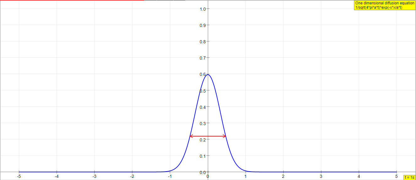
The simulation demonstrates the analytic solution of the one dimensional diffusion equation. A delta pulse at the origin is set as the initial function. This setup approximately models the temperature increase in a thin, long wire that is heated at the origin by a short laser pulse.

The analytic solution is a Gaussian spreading in time. Its integral is constant, which means that the laser pulse heating energy is conserved in the diffusion process.

To avoid the singularity of the delta function at time t = 0 the calculation starts at t = 0.0001 sec with a Gaussian of corresponding narrowness. It is visible as a blue line before start.

After Start the maximum amplitude (temperature) falls at a decreasing rate (observe the changing scale), while the width of the distribution grows correspondingly.

Arrows indicate the 1/e width. Time t is counted in an number field in seconds.

A slider defines the diffusion constant (heat conductivity) within a wide range.

One dimensional diffusion equation

∂Φ/∂t = a ∂²Φ/∂t²

With normalized delta function as initial function

Φ(0,0)  = δ(0) = 0 for x≠0       and ∫δdx = 1

the analytic solution is a normalized Gaussian function. 

Φ(x,t) = exp(-x²/at) / sqrt (4πat)

1/e- width:  at

maximum amplitude: 1 / sqrt (4πat)

E1: Measure the time dependence of the maximum amplitude and draw its graph on log-linear paper. Choose an appropriate diffusion constant and consider the changing scale.

E2: Do the same for the 1/e width of the distribution. Use a log-quadratic system for drawing, too.

E3: Interpret your measurement by analysis of the Gaussian formula.

 

Translations

Code	Language		Translator	Run

Credits

dieter.roess@t-onlione.de; Fremont Teng; Loo Kang Wee

Overview:

This document provides a briefing on the "One Dimensional Diffusion Equation JavaScript Simulation Applet HTML5" resource hosted on the Open Educational Resources / Open Source Physics @ Singapore website. This resource offers an interactive simulation to visualize and understand the analytic solution of the one-dimensional diffusion equation. It is presented as a learning tool for mathematics, specifically within the context of differential equations and their applications in physics.

Main Themes and Important Ideas/Facts:

1. Simulation of the Diffusion Equation: The core of the resource is a JavaScript simulation applet built using HTML5. This allows users to interact with a visual representation of the one-dimensional diffusion equation's analytic solution. The resource emphasizes the use of simulations for learning and teaching mathematics, particularly in relation to physics.

• Quote: "The simulation demonstrates the analytic solution of the one dimensional diffusion equation."

1. Modeling a Physical Phenomenon: The simulation is framed within a relatable physical context. It models the temperature increase in a thin, long wire heated at a single point (the origin) by a short laser pulse. This helps to connect the abstract mathematical concept of diffusion to a real-world scenario.

• Quote: "This setup approximately models the temperature increase in a thin, long wire that is heated at the origin by a short laser pulse."

1. Analytic Solution and Gaussian Spreading: The resource explicitly states that the analytic solution to the diffusion equation under these initial conditions is a Gaussian function that spreads over time. Key properties of this Gaussian distribution are highlighted:

• Quote: "The analytic solution is a Gaussian spreading in time."
• The integral of the Gaussian is constant, signifying the conservation of energy in the modeled system ("Its integral is constant, which means that the laser pulse heating energy is conserved in the diffusion process.").

1. Handling the Initial Singularity: The simulation addresses the mathematical challenge of the delta function at t = 0 (representing the instantaneous laser pulse) by starting the calculation at a very small time (t = 0.0001 sec) with a narrow Gaussian. This avoids the singularity while still approximating the initial condition.

• Quote: "To avoid the singularity of the delta function at time t = 0 the calculation starts at t = 0.0001 sec with a Gaussian of corresponding narrowness."

1. Visual Representation and Interactive Elements: The simulation provides a visual representation of the Gaussian spreading as a blue line initially. After the simulation starts, the changes in the distribution are shown, with:

• The maximum amplitude (temperature) decreasing over time.
• The width of the distribution increasing over time.
• Arrows indicating the 1/e width of the Gaussian.
• A number field displaying the elapsed time in seconds.
• A slider allowing users to adjust the diffusion constant (heat conductivity), which influences the rate of diffusion.
• Quote: "After Start the maximum amplitude (temperature) falls at a decreasing rate (observe the changing scale), while the width of the distribution grows correspondingly."
• Quote: "A slider defines the diffusion constant (heat conductivity) within a wide range."

1. Mathematical Formulation: The resource provides the formula for the one-dimensional diffusion equation and its analytic solution with a normalized delta function as the initial condition:

• Diffusion Equation: ∂Φ/∂t = a ∂2Φ/∂t2
• Initial Condition: Φ(0,0) = δ(0) = 0 for x≠0 and ∫ δdx = 1
• Analytic Solution: Φ(x,t) = exp(-x2 /4at) / sqrt (4πat) (Note: There appears to be a slight typo in the original source, the term in the exponent should likely be divided by 4*at, not at. Assuming this is a minor error.)
• 1/e- width: sqrt(4at) (Note: The source states "at", this is likely another minor typo and should be the square root for standard Gaussian width definition.)
• Maximum amplitude: 1 / sqrt (4πat)

1. Suggested Experiments: The resource includes three suggested experiments (E1, E2, E3) designed to guide users in exploring the behavior of the simulation and relating it back to the mathematical formula. These experiments involve:

• Measuring the time dependence of the maximum amplitude and plotting it on log-linear paper.
• Measuring the time dependence of the 1/e width and plotting it on log-quadratic paper.
• Interpreting the measurements through analysis of the Gaussian formula.

1. For Teachers: The resource includes a section specifically for teachers, providing instructions on how to use the "Diffusion Constant Slider" and the "Play/Pause, Step and Reset Buttons." It also mentions the ability to toggle full screen.
2. Integration and Sharing: The resource provides an Embed code (<iframe>) allowing users to easily integrate the simulation into other webpages.
3. Context within the Website: The resource is located within a section dedicated to "Pure Mathematics" under the broader category of "Interactive Resources" on the "Open Educational Resources / Open Source Physics @ Singapore" website. This suggests a focus on using interactive tools for teaching and learning STEM subjects. The extensive list of other available applets on various physics and mathematics topics further reinforces this theme.
4. Licensing and Credits: The content is licensed under a Creative Commons Attribution-Share Alike 4.0 Singapore License. Credits are given to Fremont Teng and Loo Kang Wee. Information regarding commercial use of the EasyJavaScriptSimulations Library is also provided.

Key Takeaways:

• This resource provides a valuable interactive tool for visualizing and understanding the one-dimensional diffusion equation and its Gaussian solution.
• It effectively connects abstract mathematical concepts to a concrete physical model (heat diffusion in a wire).
• The simulation allows for exploration of the impact of the diffusion constant on the spreading of the distribution.
• The suggested experiments encourage active learning and quantitative analysis of the simulation's behavior.
• The embeddable nature of the applet makes it easily shareable and integrable into educational materials.

This simulation applet appears to be a well-designed educational resource that can enhance the learning experience for students studying differential equations, heat transfer, or related physics and mathematics topics.

 

Study Guide: One Dimensional Diffusion Equation Simulation

Core Concepts

• Diffusion Equation: Understand the partial differential equation ∂Φ/∂t = a ∂²Φ/∂x², which describes how a quantity Φ spreads out over time due to a diffusion process.
• Analytic Solution: Recognize that the simulation demonstrates the exact mathematical solution to the diffusion equation for a specific initial condition.
• Initial Condition: Understand that the simulation starts with a delta pulse at the origin, approximating a localized source of heat energy.
• Gaussian Function: Know that the analytic solution to the diffusion equation with a delta pulse initial condition is a Gaussian function. Understand the general shape and properties of a Gaussian curve.
• Diffusion Constant (a): Understand that this constant represents the rate at which diffusion occurs (in this context, heat conductivity). A higher value of a means faster diffusion.
• Conservation of Energy: Recognize that the integral of the Gaussian function (representing the total heating energy) remains constant over time, indicating energy conservation.
• Temporal Evolution: Observe how the Gaussian distribution changes over time: the maximum amplitude decreases, and the width increases.
• 1/e Width: Understand that the arrows in the simulation indicate the width of the distribution at 1/e of its maximum amplitude and that this width is related to the diffusion constant and time by the formula √(4at).
• Maximum Amplitude: Understand that the maximum amplitude of the Gaussian distribution changes over time according to the formula 1 / √(4πat).
• Simulation Controls: Familiarize yourself with the function of the diffusion constant slider, the play/pause, step, and reset buttons, and the time display.
• Modeling a Physical System: Understand how the simulation approximates the temperature increase in a thin wire heated by a short laser pulse.

Quiz

1. What physical scenario does this simulation approximately model?
2. Describe the initial condition of the simulation. What mathematical function represents this condition?
3. What type of mathematical function is the analytic solution to the one-dimensional diffusion equation with the given initial condition? How does its shape change over time in the simulation?
4. What does the diffusion constant (a) represent in the context of this simulation? How does changing its value affect the diffusion process?
5. What does it mean that the integral of the analytic solution is constant? What physical principle does this illustrate?
6. Describe how the maximum amplitude of the Gaussian distribution changes as time progresses in the simulation. What is the mathematical relationship for this change?
7. What do the arrows in the simulation indicate? What is the formula for this width?
8. Why does the simulation start the calculation at t = 0.0001 seconds instead of t = 0?
9. Explain the purpose of the experiments (E1, E2, E3) suggested in the description. What kind of analysis are they designed to encourage?
10. How can the simulation be embedded in a webpage? What HTML element is used for this purpose?

Quiz Answer Key

1. The simulation approximately models the temperature increase in a thin, long wire that is heated at the origin by a short laser pulse. The initial localized heating spreads out along the wire over time.
2. The initial condition is a delta pulse at the origin, which is represented mathematically by the Dirac delta function, δ(0). In the simulation, to avoid singularity at t=0, it starts with a very narrow Gaussian.
3. The analytic solution is a normalized Gaussian function. Over time, the Gaussian broadens (its width increases) while its peak amplitude decreases, maintaining a constant area under the curve.
4. The diffusion constant (a) represents the rate of diffusion, which in this model corresponds to the heat conductivity of the wire. A higher diffusion constant results in a faster spread of the temperature distribution.
5. The constant integral signifies that the total amount of the diffusing quantity (in this case, the laser pulse heating energy) is conserved throughout the diffusion process; it is just spreading out.
6. The maximum amplitude of the Gaussian distribution decreases over time at a decreasing rate. Mathematically, it is inversely proportional to the square root of time: 1 / √(4πat).
7. The arrows indicate the 1/e width of the Gaussian distribution. The formula for this width is √(4at).
8. The simulation starts at a small non-zero time to avoid the singularity of the delta function at t = 0, where its amplitude would be infinite. It uses a very narrow Gaussian as an approximation at this early time.
9. The experiments are designed to encourage the user to analyze the time dependence of the maximum amplitude and the 1/e width by plotting the measured data on different types of graph paper and interpreting the results based on the provided Gaussian formula.
10. The simulation can be embedded in a webpage using an <iframe> HTML element, with the src attribute pointing to the simulation's URL.

Essay Format Questions

1. Discuss the physical significance of the one-dimensional diffusion equation and how the simulation effectively illustrates its analytic solution for a delta pulse initial condition. Consider the concepts of heat transfer and energy conservation in your response.
2. Analyze the relationship between the diffusion constant, time, the maximum amplitude, and the width of the Gaussian distribution as demonstrated by the simulation and its corresponding formulas. Explain how changing the diffusion constant affects the temporal evolution of the temperature profile.
3. Describe the process of modeling a physical phenomenon using a mathematical equation and a simulation. Using the example of the heated wire, discuss the approximations made in the model and the benefits of using a simulation to visualize the abstract mathematical solution.
4. Evaluate the pedagogical value of this interactive simulation for learning about the one-dimensional diffusion equation. How do the visual representation and the ability to manipulate parameters (like the diffusion constant) enhance understanding compared to simply studying the mathematical formulas?
5. Consider potential extensions or modifications to this simulation that could explore more complex diffusion scenarios, such as different initial conditions, boundary conditions, or variations in the diffusion constant. How might these modifications deepen the understanding of diffusion processes?

Glossary of Key Terms

• Diffusion: The net movement of a substance (e.g., heat, particles) from a region of high concentration to a region of low concentration as a result of random motion of its constituent particles.
• One-Dimensional: Involving variation in only one spatial direction. In this context, the heat spreads along the length of the thin wire.
• Diffusion Equation: A partial differential equation that describes the density of a substance as it undergoes diffusion.
• Analytic Solution: An exact mathematical solution to a differential equation expressed in terms of elementary functions or infinite series.
• Delta Pulse: A mathematical idealization representing a quantity that is concentrated at a single point in space and time, with an infinite amplitude and zero width, but a finite integral. Approximated here by a narrow Gaussian.
• Gaussian Function: A type of function characterized by its bell-shaped curve, mathematically represented as Φ(x,t) = exp(-x² / (4at)) / √(4πat) in this context.
• Diffusion Constant (a): A measure of how quickly a substance diffuses through a medium. In heat diffusion, it is related to the thermal conductivity, density, and specific heat capacity.
• Singularity: A point at which a mathematical function becomes undefined or infinite. The delta function has a singularity at its peak.
• Integral: In calculus, the area under a curve. In this context, the integral of the Gaussian represents the total amount of the diffusing quantity (energy).
• 1/e Width: A measure of the spread of the Gaussian distribution, specifically the distance between the two points where the amplitude is 1/e (approximately 37%) of the maximum amplitude.
• Maximum Amplitude: The highest value reached by the Gaussian function, located at the center of the distribution.
• Partial Differential Equation: A differential equation that contains unknown multivariable functions and their partial derivatives.
• Heat Conductivity: A measure of a material's ability to conduct heat. A higher heat conductivity means heat will diffuse more quickly.

Sample Learning Goals

[text]

For Teachers

One Dimensional Diffusion Equation JavaScript Simulation Applet HTML5

Instructions

Diffusion Constant Slider

Toggling Full Screen

Play/Pause, Step and Reset Buttons

Research

[text]

Video

[text]

 Version:

Other Resources

[text]

Frequently Asked Questions: One Dimensional Diffusion Equation Simulation

• What does this simulation demonstrate? The simulation visually demonstrates the analytic solution to the one-dimensional diffusion equation. It specifically models a scenario where a short laser pulse heats a thin, long wire at its origin, creating an initial delta pulse of temperature. The simulation then shows how this initial heat distribution spreads out over time due to diffusion.
• How is the initial condition represented in the simulation? The initial condition is a delta pulse at the origin, representing the localized heating by the laser. However, to avoid the mathematical singularity of a delta function at time t = 0, the simulation starts at a very small time (t = 0.0001 sec) with a very narrow Gaussian function that approximates the delta pulse. This initial narrow Gaussian is visible as a blue line before the simulation starts.
• What happens to the temperature distribution over time in the simulation? After the simulation starts, the initial narrow peak of temperature (represented by the Gaussian function) spreads out over time. The maximum amplitude (peak temperature) decreases, while the width of the temperature distribution increases. The rate at which the maximum amplitude falls decreases over time, and the scale of the graph adjusts to show these changes. The total "heating energy," represented by the integral of the distribution, remains constant throughout the diffusion process.
• What is the mathematical formula for the one-dimensional diffusion equation and its analytic solution in this context? The one-dimensional diffusion equation is given by ∂Φ/∂t = a ∂²Φ/∂x², where Φ represents the temperature distribution, t is time, x is the spatial dimension, and a is the diffusion constant (related to heat conductivity). With a normalized delta function as the initial condition (Φ(x,0) = δ(x)), the analytic solution is a normalized Gaussian function: Φ(x,t) = exp(-x² / (4at)) / sqrt(4πat).
• What do the arrows in the simulation indicate? The arrows in the simulation indicate the 1/e-width of the Gaussian distribution. This width is a measure of the spread of the distribution and is mathematically given by sqrt(at). As time progresses, the arrows move further apart, indicating that the heat distribution is spreading.
• How can the diffusion constant be adjusted in the simulation? The simulation includes a slider that allows the user to adjust the diffusion constant (a). This constant directly affects the rate of diffusion. A higher diffusion constant will lead to a faster spread of the heat and a quicker decrease in the maximum amplitude.
• What experiments are suggested using this simulation? Three experiments are suggested:

1. Measure the time dependence of the maximum amplitude and plot it on log-linear paper.
2. Measure the time dependence of the 1/e-width of the distribution and plot it on both log-linear and log-quadratic paper.
3. Interpret the measurements from the first two experiments by analyzing the provided Gaussian formula for the analytic solution.

• What are some key learning goals associated with this simulation? While specific learning goals are not explicitly listed in the provided text excerpt, it can be inferred that the simulation aims to help users understand the concept of diffusion, visualize the solution of a partial differential equation, observe the relationship between the diffusion constant and the rate of spreading, and analyze the mathematical form of the Gaussian distribution in the context of a physical process like heat conduction.