About

This simulation illustrates the concept of a limit cycle by using the following mathematical model:

dx/dt = y +  [K*x*(1 - x^2 - y^2)]/sqrt(x^2 +  y^2)

dy/dt = -x + [K*y*(1 - x^2 - y^2)]/sqrt(x^2 +  y^2)

The initial conditions are as follows:

x(0) = x0

y(0) = y0

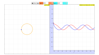
The limit cycle of this function is a circle centered at the origin with radius 1 (the unit circle), which can be expressed in the following statement.

For all x0,y0 (where x0, y0 are non-zero), x^2 + y^2 approaches 1 as t tends to infinity.

The initial value conditions in the XY-plane can be set by using two sliders and fields. Press the "Initialize", then "Play" button to start the simulation. The model trajectory is displayed. Alfonso Urquía and Carla Martín
Dpto. de Informática y Automática
E.T.S. Ingeniería Informática, UNED
Juan del Rosal 16, 28040 Madrid, Spain  

Translations

Code	Language		Translator	Run

Credits

Alfonso Urquía; Carla Martín; Tan Wei Chiong; Loo Kang Wee

• sustaining oscillation.
• Mathematical Model: A description of a system using mathematical language. In this case, it's a pair of differential equations describing the rate of change of x and y coordinates.
• Differential Equations: Equations that relate a function with its derivatives. The provided model uses first-order ordinary differential equations.
• Initial Conditions: The starting values of the variables at a specific time (t=0). Here, they are denoted as x(0) = x0 and y(0) = y0.
• Phase Space (XY-plane): A plane where the axes represent the state variables of the system (here, x and y). The trajectory of the system is plotted in this plane.
• Trajectory: The path traced by a point in the phase space as time evolves, determined by the governing equations and initial conditions.
• Unit Circle: A circle centered at the origin (0,0) with a radius of 1, defined by the equation x² + y² = 1.
• Approach as t tends to infinity: Describes the long-term behavior of the system, indicating what happens to the variables as time progresses indefinitely.

Quiz

1. What is a limit cycle, as illustrated by this simulation?
2. Write down the mathematical model used in this simulation to describe the limit cycle.
3. What are the initial conditions that can be set in the simulation? How can these be adjusted in the applet?
4. According to the description, what is the specific limit cycle of the given mathematical model?
5. Explain the statement "For all x0,y0 (where x0, y0 are non-zero), x^2 + y^2 approaches 1 as t tends to infinity" in your own words.
6. What does the graph on the left of the simulation typically illustrate? What about the graph on the right?
7. Identify the authors credited with the development of this simulation model.
8. What programming language is this simulation applet written in? What does HTML5 signify in this context?
9. Where can this simulation model be embedded, according to the provided text?
10. Besides this limit cycle simulation, name two other interactive resources listed on the same webpage.

Answer Key for Quiz

1. A limit cycle in this simulation is a stable, closed path in the XY-plane (the unit circle) that the trajectory of any non-zero initial condition will eventually spiral towards as time goes on. It represents a sustained oscillation that the system settles into regardless of its starting point.
2. The mathematical model is given by the following pair of differential equations: dx/dt = y + [Kx(1 - x^2 - y^2)]/sqrt(x^2 + y^2) and dy/dt = -x + [Ky(1 - x^2 - y^2)]/sqrt(x^2 + y^2). The initial conditions are x(0) = x0 and y(0) = y0.
3. The initial conditions are the starting values for the x and y coordinates at time t=0, denoted as x0 and y0. These can be set in the simulation using two sliders and corresponding input fields provided in the applet interface.
4. The limit cycle of this specific function is a circle centered at the origin of the XY-plane with a radius of 1, which is also known as the unit circle. This is defined by the equation x² + y² = 1.
5. This statement means that no matter where you start on the XY-plane (as long as it's not exactly at the origin), if you let the system evolve according to the given differential equations for a very long time, the values of x and y will change such that the point (x, y) gets arbitrarily close to lying on the unit circle.
6. The graph on the left typically illustrates the trajectory of the point (x, y) in the phase space (the XY-plane), showing how it moves over time. The graph on the right illustrates the individual changes of the y-coordinate (blue line) and the x-coordinate (red line) as functions of time (t).
7. The authors credited with the development of this simulation model are Alfonso Urquía and Carla Martín from the Dpto. de Informática y Automática, E.T.S. Ingeniería Informática, UNED, Madrid, Spain.
8. This simulation applet is written in JavaScript, as indicated by the title and the nature of HTML5 applets. HTML5 is the latest evolution of the standard used to structure and present content on the World Wide Web, enabling interactive elements and multimedia without the need for separate plugins.
9. According to the text, this simulation model can be embedded in a webpage using an <iframe> tag with the provided source URL. This allows the interactive simulation to be displayed directly within another HTML document.
10. Two other interactive resources listed on the same webpage include "Monte Carlo Pi Calculation JavaScript Simulation Applet HTML5" and "Ball and Beam JavaScript Simulation Applet HTML5" (many others are listed as well).

Essay Format Questions

1. Discuss the significance of the mathematical model provided in accurately representing the behavior of the limit cycle. How do the differential equations define the system's evolution towards the unit circle?
2. Explain the relationship between the initial conditions and the eventual trajectory of the system in the context of a limit cycle. Why does the system always approach the same limit cycle regardless of the non-zero starting point?
3. Describe how the interactive features of the JavaScript simulation applet enhance the understanding of the abstract concept of a limit cycle. What specific actions can a user take and what visual feedback does the applet provide?
4. Consider the broader context of differential equations and dynamical systems. How does the concept of a limit cycle fit into the study of oscillations and stability in such systems?
5. Based on the provided information and the nature of open educational resources, discuss the potential benefits and applications of such interactive simulations in teaching and learning mathematical concepts like limit cycles and differential equations.

Glossary of Key Terms

• Calculus: A branch of mathematics that deals with continuous change, involving concepts like derivatives, integrals, limits, and infinite series. It is fundamental to understanding rates of change and accumulation.

Limit Cycle Simulation Study Guide

Key Concepts

• Limit Cycle: A closed trajectory in the phase space having the property that other trajectories starting sufficiently close to it (both inside and outside) spiral into it as time approaches infinity. It represents a self-sustaining oscillation.
• Mathematical Model: A description of a system using mathematical language. In this case, it's a pair of differential equations describing the rate of change of x and y coordinates.
• Differential Equations: Equations that relate a function with its derivatives. The provided model uses first-order ordinary differential equations.
• Initial Conditions: The starting values of the variables at a specific time (t=0). Here, they are denoted as x(0) = x0 and y(0) = y0.
• Phase Space (XY-plane): A plane where the axes represent the state variables of the system (here, x and y). The trajectory of the system is plotted in this plane.
• Trajectory: The path traced by a point in the phase space as time evolves, determined by the governing equations and initial conditions.
• Unit Circle: A circle centered at the origin (0,0) with a radius of 1, defined by the equation x² + y² = 1.
• Approach as t tends to infinity: Describes the long-term behavior of the system, indicating what happens to the variables as time progresses indefinitely.

Quiz

1. What is a limit cycle, as illustrated by this simulation?
2. Write down the mathematical model used in this simulation to describe the limit cycle.
3. What are the initial conditions that can be set in the simulation? How can these be adjusted in the applet?
4. According to the description, what is the specific limit cycle of the given mathematical model?
5. Explain the statement "For all x0,y0 (where x0, y0 are non-zero), x^2 + y^2 approaches 1 as t tends to infinity" in your own words.
6. What does the graph on the left of the simulation typically illustrate? What about the graph on the right?
7. Identify the authors credited with the development of this simulation model.
8. What programming language is this simulation applet written in? What does HTML5 signify in this context?
9. Where can this simulation model be embedded, according to the provided text?
10. Besides this limit cycle simulation, name two other interactive resources listed on the same webpage.

Answer Key for Quiz

1. A limit cycle in this simulation is a stable, closed path in the XY-plane (the unit circle) that the trajectory of any non-zero initial condition will eventually spiral towards as time goes on. It represents a sustained oscillation that the system settles into regardless of its starting point.
2. The mathematical model is given by the following pair of differential equations: dx/dt = y + [Kx(1 - x^2 - y^2)]/sqrt(x^2 + y^2) and dy/dt = -x + [Ky(1 - x^2 - y^2)]/sqrt(x^2 + y^2). The initial conditions are x(0) = x0 and y(0) = y0.
3. The initial conditions are the starting values for the x and y coordinates at time t=0, denoted as x0 and y0. These can be set in the simulation using two sliders and corresponding input fields provided in the applet interface.
4. The limit cycle of this specific function is a circle centered at the origin of the XY-plane with a radius of 1, which is also known as the unit circle. This is defined by the equation x² + y² = 1.
5. This statement means that no matter where you start on the XY-plane (as long as it's not exactly at the origin), if you let the system evolve according to the given differential equations for a very long time, the values of x and y will change such that the point (x, y) gets arbitrarily close to lying on the unit circle.
6. The graph on the left typically illustrates the trajectory of the point (x, y) in the phase space (the XY-plane), showing how it moves over time. The graph on the right illustrates the individual changes of the y-coordinate (blue line) and the x-coordinate (red line) as functions of time (t).
7. The authors credited with the development of this simulation model are Alfonso Urquía and Carla Martín from the Dpto. de Informática y Automática, E.T.S. Ingeniería Informática, UNED, Madrid, Spain.
8. This simulation applet is written in JavaScript, as indicated by the title and the nature of HTML5 applets. HTML5 is the latest evolution of the standard used to structure and present content on the World Wide Web, enabling interactive elements and multimedia without the need for separate plugins.
9. According to the text, this simulation model can be embedded in a webpage using an <iframe> tag with the provided source URL. This allows the interactive simulation to be displayed directly within another HTML document.
10. Two other interactive resources listed on the same webpage include "Monte Carlo Pi Calculation JavaScript Simulation Applet HTML5" and "Ball and Beam JavaScript Simulation Applet HTML5" (many others are listed as well).

Essay Format Questions

1. Discuss the significance of the mathematical model provided in accurately representing the behavior of the limit cycle. How do the differential equations define the system's evolution towards the unit circle?
2. Explain the relationship between the initial conditions and the eventual trajectory of the system in the context of a limit cycle. Why does the system always approach the same limit cycle regardless of the non-zero starting point?
3. Describe how the interactive features of the JavaScript simulation applet enhance the understanding of the abstract concept of a limit cycle. What specific actions can a user take and what visual feedback does the applet provide?
4. Consider the broader context of differential equations and dynamical systems. How does the concept of a limit cycle fit into the study of oscillations and stability in such systems?
5. Based on the provided information and the nature of open educational resources, discuss the potential benefits and applications of such interactive simulations in teaching and learning mathematical concepts like limit cycles and differential equations.

Glossary of Key Terms

• Calculus: A branch of mathematics that deals with continuous change, involving concepts like derivatives, integrals, limits, and infinite series. It is fundamental to understanding rates of change and accumulation.
• Differential Equation: A mathematical equation that relates a function with its derivatives. These equations are used to model processes that change over time or space.
• JavaScript: A high-level, often just-in-time compiled programming language that conforms to the ECMAScript specification. It is commonly used in web browsers to make web pages interactive.
• HTML5: The latest evolution of the standard that defines the structure and content of the World Wide Web. It includes features for multimedia and interactive elements without requiring plugins.
• Simulation: A computerized model that mimics the behavior of a real-world system or process over time, allowing users to observe and interact with it.
• Applet: A small application, often written in Java or JavaScript, that runs within another application, typically a web browser, to provide interactive functionality.
• Open Educational Resources (OER): Teaching, learning, and research materials that are freely available and can be reused, remixed, revised, and redistributed with no or minimal restrictions.
• Ordinary Differential Equation (ODE): A differential equation containing one or more functions of one independent variable and their derivatives with respect to that variable. The equations in the model are ODEs where time (t) is the independent variable.
• Phase Space: A space in which all possible states of a system are represented, with each possible state corresponding to one unique point in the phase space. For a system with variables x and y, the phase space is often the XY-plane.
• Trajectory (in phase space): The path traced out by a point representing the state of a dynamical system as time evolves in the phase space.

Sample Learning Goals

[text]

For Teachers

This simulation illustrates the concept of a limit cycle by using the following mathematical model:
dx/dt = y + [K*x*(1 - x^2 - y^2)]/sqrt(x^2 + y^2)
dy/dt = -x + [K*y*(1 - x^2 - y^2)]/sqrt(x^2 + y^2)

The initial conditions are as follows:
x(0) = x0
y(0) = y0

The limit cycle of this function is a circle centered at the origin with radius 1 (the unit circle), which can be expressed in the following statement.
For all x0,y0 (where x0, y0 are non-zero), x^2 + y^2 approaches 1 as t tends to infinity.

In essence, for any point on the Cartesian plane, it will eventually approach the limit of the unit circle, no matter where the point is.

The graph on the left illustrates the path of the point, while the graph on the right illustrates the graph of y against t (blue) and x against t (red).

Research

[text]

Video

[text]

 Version:

1. http://weelookang.blogspot.com/2018/05/limit-cycle-javascript-simulation.html 
   
2. http://www.euclides.dia.uned.es/simulab-pfp/curso_online/cap7_caseStudies/leccion.htm by Alfonso Urquia and Carla Martin-Villalba

Other Resources

[text]

Frequently Asked Questions: Limit Cycle Simulation

1. What is a limit cycle, and how does this simulation illustrate it?

A limit cycle is an isolated closed trajectory in the phase space having the property that at least one other trajectory spirals into it as time approaches infinity or minus infinity. This JavaScript simulation illustrates this concept through a mathematical model defined by two differential equations. Regardless of the non-zero initial conditions set in the XY-plane, the plotted trajectory of the system approaches a circle of radius 1 centered at the origin, which is the limit cycle in this specific model.

2. What is the mathematical model used in this simulation?

The simulation utilizes the following system of ordinary differential equations:

• dx/dt = y + [Kx(1 - x^2 - y^2)http://weelookang.blogspot.com/2018/05/limit-cycle-javascript-simulation.html
• http://www.euclides.dia.uned.es/simulab-pfp/curso_online/cap7_caseStudies/leccion.htm by Alfonso Urquia and Carla Martin-Villalba These links might offer slightly different interfaces or additional context related to the limit cycle phenomenon.