About

Definite integral

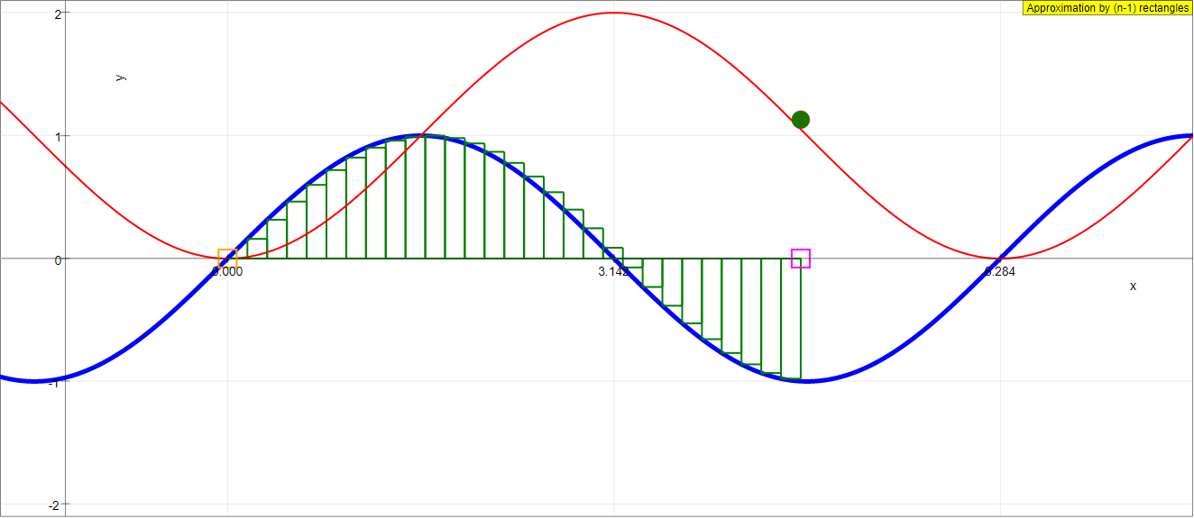
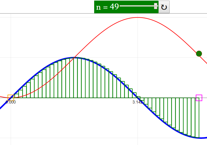
This simulation demonstrates definite integration of the sine function by the simple algorithm of summing approximative rectangles. The red curve shows the sine function itself.

The definite integral is to be calculated between initial point x₁ (blue) an end point x₂ (magenta). A first slider defines x₁ ; x₂ can be drawn with the mouse.

The red curve is the analytic antiderivative for an initial value x₁: y = cos(x) - cos (x1).

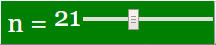
A second slider n defines the number n-1 of subinterval into which x₂ - x₁ is divided for the approximation. In each subinterval the approximative amplitude is assumed to be equal to its initial value. The sum of the area of all rectangles is shown by a green point at x₂ .

Reset defines 1 < x < 4 and n-1 = 9.

E1: Start with the default setting: x1 = 0; n = 10.

Draw the magenta end point and observe the deviation of the rectangle sum (green point) from the analytic solution.

E2: Understand why the deviation is negative for x < π/2, and why it becomes zero at x = π . Reflect how summing mistakes can compensate for periodic functions.

E3: Increase the number of intervals with the slider and observe how the deviation changes and disappears in the limit.

E4: Change the initial point and consider why and how this shifts the analytic solution.

E5: Choose a large integration interval and consider why the rectangles lie below or above certain parts of the function.

 

Translations

Code	Language		Translator	Run

Credits

Dieter Roess - WEH-Foundation; Fremont Teng; Loo Kang Wee

Sample Learning Goals

[text]

For Teachers

Definite Integral JavaScript Simulation Applet HTML5

Instructions

N Slider

Draggable Boxes

Toggling Full Screen

Reset Button

Research

[text]

Video

[text]

 Version:

Other Resources

[text]

end faq

{accordionfaq faqid=accordion4 faqclass="lightnessfaq defaulticon headerbackground headerborder contentbackground contentborder round5"}