Breadcrumbs

About

Intro Page

Integral: algorithms of numerical approximation

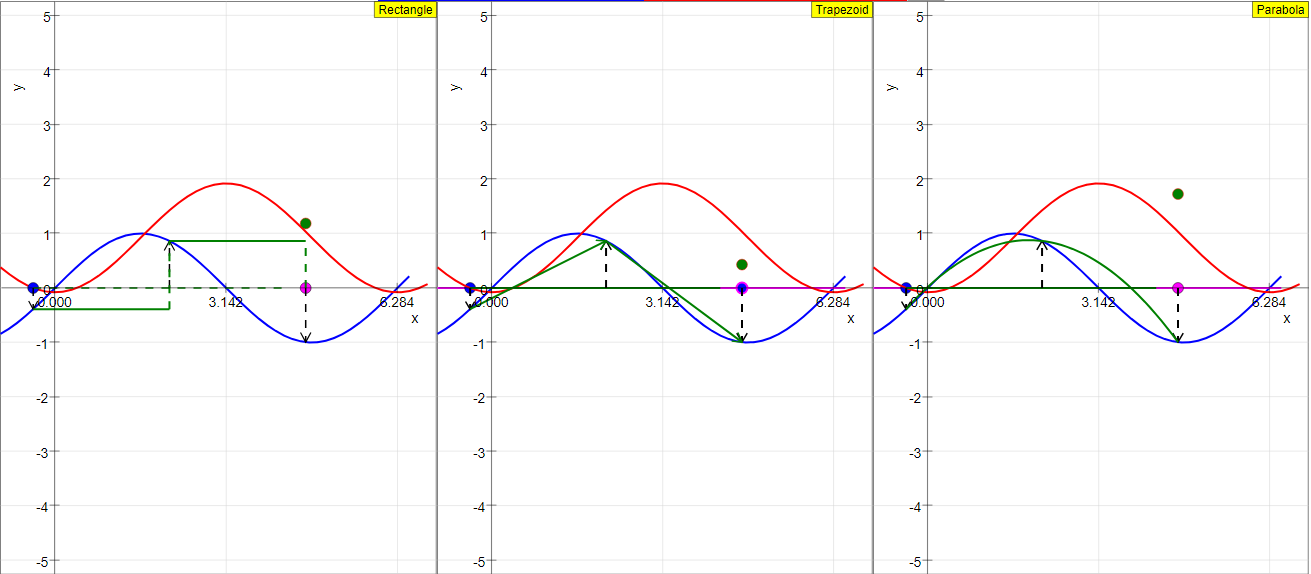
As an example for numerical integration we choose the sine function y = sin x ; its graph is shown in blue. The definite integral is to be calculated between an initial abscissa x₁ and an end abscissa x₂.

The analytic solution of the indefinite integral (antiderivative) is

y = ∫ sinxdx = -cos x +C

Its graph is shown in red, with C as the initial value at the initial abscissa.

The analytic definite integral is -(cos x₂-cosx₁). It corresponds to a point on the analytic curve at the end abscissa x₂.

In the approximate numerical calculation the interval x₂- x₁ is divided into n sub intervals of width delta. For clear demonstration of the principle n = 2 is chosen. Arrows show the value of the function in the three points of the double interval 2 delta.

Three numerical algorithms are visualized in three windows. They differ in how the approximative value of the function is defined between consecutive points in the sub interval delta.

1.) Rectangle approximation: y is taken as constant within the interval. The contribution of one interval is delta * y₁.

2.) Trapezoid approximation: y is taken as the mean value within the interval. Its contribution is delta*(y₁+y₂)/2.

3.) Parabola approximation: the function in two consecutive intervals is approximated by a second order parabola through both end points and the middle point of the double interval (a parabola needs three points to be uniquely defined). The contribution of the double integral, derived as a surprisingly simple formula, is 2*delta*1/6(y₁+4y₂+y₃).

In principle one can increase the precision of the parabola algorithm still further by using higher order parabolas, with correspondingly more sub intervals of the definition range. As the second order is already very good, higher order approximations have no great practical importance. (For fun and exercise derive the formula for a third order parabola!)

The simulation calculates the sum of two approximating intervals of width delta using the three algorithms. Their respective values are represented by the green points.

A first slider defines the interval delta, a second one the initial abscissa x₁, reset defines delta = 1 and x₁ = 0.5.

Experiments

E1: Start with the default values : x₁= 0.5; delta=1

Compare how well the three procedures approximate the analytic solution.

E2: Draw the initial value with the mouse. Observe the shift of the analytic solution, and its relation to the result of the different algorithms. Explain mentally to some non professional what you observe!

E4: Reduce the interval width and observe how fast the approximations converge to the analytic solution.

E4: Keep the interval small and approximately constant while drawing the initial point. Observe whether the differences of the algorithms are comparable for all initial points. Interpret the result!

E5: For special initial points the simple algorithms result in exact agreement with the analytic value, while the parabola algorithms shows a recognizable deviation. Does this mean that the simple ones are better? What is the reason for identity in these cases?

Translations

Code	Language		Translator	Run

Credits

Dieter Roess - WEH-Foundation; Fremont Teng; Loo Kang Wee

This resource provides an interactive simulation designed to illustrate and compare different numerical methods for approximating definite integrals.

2. Main Themes and Important Ideas:

The central theme of this resource is the concept of numerical integration as an approximation technique for definite integrals. The simulation focuses on visually demonstrating and comparing three common numerical approximation algorithms:

Rectangle Approximation: Approximating the area under a curve by summing the areas of rectangles whose heights are determined by the function value at either the left, right, or midpoint of each subinterval. The resource explicitly states: " y is taken as constant within the interval. The contribution of one interval is delta * y1."
Trapezoid Approximation: Approximating the area under a curve by summing the areas of trapezoids formed by connecting consecutive points on the curve with straight lines. The resource explains: "y is taken as the mean value within the interval. Its contribution is delta*(y1+y2 )/2."
Parabola Approximation (Simpson's Rule in essence): Approximating the curve over pairs of subintervals with a second-order parabola. The area under the parabola is then used to estimate the definite integral. The resource details: "the function in twoconsecutive intervals is approximated by a second order parabola through both end points and the middle point of the double interval... The contribution of the double integral... is 2delta1/6(y1+4y2+y3 *)."

Key Important Ideas:

Definite vs. Indefinite Integrals: The resource clearly distinguishes between the indefinite integral (antiderivative) with its analytic solution y = ∫ sinxdx = -cos x +C and the definite integral which is calculated between specific limits x1 and x2.
Numerical Approximation: The need for numerical methods arises when an analytic solution to a definite integral is difficult or impossible to find. The simulation demonstrates how these methods provide approximate values.
Subintervals and Delta: The accuracy of numerical integration generally increases as the interval x2 - x1 is divided into a larger number (n) of smaller subintervals of width delta. The simulation allows users to adjust delta and observe the impact on the approximations.
Convergence: The resource implicitly addresses the idea of convergence, suggesting that as the interval width (delta) decreases, the numerical approximations should get closer to the analytic solution. Experiment E4 explicitly prompts the user to "Reduce the interval width and observe how fast the approximations converge to the analytic solution."
Accuracy and Choice of Algorithm: The simulation visually highlights that different numerical algorithms offer varying levels of accuracy for the same function and interval. The parabola approximation is presented as generally more accurate than the rectangle and trapezoid methods for a given number of subintervals. The text notes, "As the second order is already very good, higher order approximations have no great practical importance."
Visual Demonstration: The JavaScript simulation allows users to interact with the parameters (initial abscissa x1 and interval width delta) and observe in real-time how the different approximation methods compare to the analytic solution of the definite integral of y = sin x. The green points in the simulation represent the values calculated by the three algorithms.
Learning by Experimentation: The "Experiments" section encourages active learning by guiding users through specific scenarios to observe the behavior of the different algorithms under varying conditions.

3. Key Facts and Details:

Example Function: The simulation uses the sine function, y = sin x, as the example function for numerical integration.
Analytic Solution: The analytic indefinite integral is given as y = ∫ sinxdx = -cos x +C, and the definite integral as -(cos x2-cosx1).
Number of Subintervals: For clear demonstration, the simulation initially uses n = 2 subintervals.
User Controls: The simulation features two sliders to adjust the interval width (delta) and the initial abscissa (x1). A "reset" button sets delta = 1 and x1 = 0.5.
Visualization: Three separate windows visually represent the rectangle, trapezoid, and parabola approximations. Arrows indicate the function values at relevant points.
Embeddability: The simulation can be embedded in other webpages using an provided iframe code.
Credits: The resource credits Dieter Roess, Fremont Teng, and Loo Kang Wee for its creation.
Licensing: The content is licensed under the Creative Commons Attribution-Share Alike 4.0 Singapore License. Commercial use of the EasyJavaScriptSimulations Library requires a separate license.
Related Resources: The page includes an extensive list of other interactive JavaScript simulations covering various topics in physics and mathematics, indicating a broader collection of open educational resources from this source.

4. Notable Quotes:

On Rectangle Approximation: " y is taken as constant within the interval. The contribution of one interval is delta * y1."
On Trapezoid Approximation: "y is taken as the mean value within the interval. Its contribution is delta*(y1+y2 )/2."
On Parabola Approximation: "the contribution of the double integral... is 2delta1/6(y1+4y2+y3 *)."
On Higher Order Approximations: "As the second order is already very good, higher order approximations have no great practical importance."
On the Simulation's Purpose: "The simulation calculates the sum of two approximating intervals of width delta using the three algorithms. Their respective values are represented by the green points."

5. Potential Implications and Use:

This simulation applet is a valuable tool for:

Mathematics Education: It provides a visual and interactive way for students to understand the concepts of numerical integration and compare different approximation methods.
Calculus Instruction: It can be used by instructors to demonstrate these concepts in the classroom and assign interactive exercises to students.
Self-Learning: Individuals can use the simulation to explore numerical integration at their own pace and develop an intuitive understanding of the algorithms.
Open Educational Resources: It contributes to the growing collection of freely accessible educational materials in mathematics and physics.

The "Experiments" section offers structured learning activities that encourage critical thinking and observation. For example, Experiment E5 prompts users to consider scenarios where simpler algorithms might coincidentally produce exact results, leading to a deeper understanding of the strengths and limitations of each method.

6. Conclusion:

The "Integral: Algorithms of Numerical Approximation JavaScript Simulation Applet HTML5" is a well-designed and effective educational resource. Its interactive nature, clear visualizations, and guided experiments make it an excellent tool for learning and teaching numerical integration. The comparison of three common algorithms, along with the ability to manipulate key parameters, provides a strong foundation for understanding this important topic in calculus. The extensive list of other simulations on the website further highlights the valuable contributions of Open Educational Resources / Open Source Physics @ Singapore to STEM education.

Key Concepts

Definite Integral: The definite integral of a function over a specified interval represents the signed area between the curve of the function and the x-axis within those limits.
Indefinite Integral (Antiderivative): A function whose derivative is the original function. The indefinite integral includes an arbitrary constant of integration, denoted by C.
Analytic Solution: A closed-form expression for the exact value of an integral, often found using the antiderivative of the function.
Numerical Approximation: Techniques used to estimate the value of a definite integral when an analytic solution is difficult or impossible to find, by dividing the area into simpler shapes.
Subintervals: Smaller intervals created by dividing the total interval of integration into n parts.
Delta (Δ): The width of each subinterval, calculated as (x2 - x1) / n.
Rectangle Approximation: A numerical integration method where the area under the curve in each subinterval is approximated by a rectangle whose height is the function's value at either the left endpoint, right endpoint, or midpoint of the subinterval. The source material uses the left endpoint.
Trapezoid Approximation: A numerical integration method where the area under the curve in each subinterval is approximated by a trapezoid whose parallel sides are the function's values at the endpoints of the subinterval.
Parabola Approximation (Simpson's Rule for n=2): A numerical integration method that approximates the curve over two consecutive subintervals using a second-order parabola passing through the endpoints and the midpoint of the combined interval.
Simulation: An interactive computer program that models a process or system, allowing users to explore different parameters and observe the results.
Convergence: The tendency of a numerical approximation to approach the exact value as the number of subintervals (n) increases (and the width of each subinterval, Δ, decreases).

Quiz

What is the difference between a definite integral and an indefinite integral? Explain their respective roles in calculus as described in the source.
Describe the core idea behind numerical approximation of a definite integral. Why is it sometimes necessary to use numerical methods instead of finding an analytic solution?
Explain how the interval [x1, x2] is divided in the process of numerical integration as described in the source. What does the variable 'delta' represent in this process?
Outline the rectangle approximation method for numerical integration as presented in the source. How is the contribution of a single subinterval calculated in this method?
Describe the trapezoid approximation method. How does it differ from the rectangle approximation in estimating the area within a subinterval?
Explain the parabola approximation method detailed in the source. Why does it require considering two consecutive intervals?
According to the source, why might the parabola approximation generally provide a better estimate than the rectangle or trapezoid approximations?
What is the purpose of the JavaScript simulation applet described in the source? How can users interact with it to explore numerical integration?
Based on Experiment E4, what happens to the accuracy of the numerical approximations when the interval width (delta) is reduced? Explain the concept of convergence in this context.
According to Experiment E5, in what specific scenarios might simpler algorithms (rectangle, trapezoid) surprisingly agree exactly with the analytic solution, while the parabola algorithm shows a deviation? What could be the reason for this?

Answer Key

A definite integral calculates the signed area under a curve between two specific limits, resulting in a numerical value. An indefinite integral, on the other hand, finds a family of functions (the antiderivative) whose derivative is the original function, including a constant of integration.
Numerical approximation estimates the definite integral by dividing the area under the curve into simpler geometric shapes (like rectangles, trapezoids, or parabolas) and summing their areas. This is needed when finding an analytic antiderivative is difficult, time-consuming, or impossible.
The interval [x1, x2] is divided into n smaller subintervals of equal width, denoted by 'delta' (Δ). Delta is calculated by subtracting the initial abscissa (x1) from the end abscissa (x2) and dividing by the number of subintervals (n). In the simulation, n is set to 2 for clear demonstration.
In the rectangle approximation, the function's value is assumed to be constant within each subinterval. The contribution of a single subinterval is calculated by multiplying the width of the subinterval (delta) by the function's value at the left endpoint (y1), resulting in an area of delta * y1.
The trapezoid approximation estimates the area in each subinterval by considering the function's values at both endpoints (y1 and y2). The contribution of a subinterval is calculated as the width (delta) multiplied by the average of the function values at the endpoints: delta * (y1 + y2) / 2.
The parabola approximation uses a second-order parabola to approximate the function over two consecutive subintervals. It requires three points: the function values at the beginning (y1), middle (y2), and end (y3) of the double interval (2delta) to uniquely define the parabola.
The parabola approximation generally offers better accuracy because it uses a higher-order polynomial to approximate the function's behavior over a small interval. By fitting a parabola, it can capture more of the curve's curvature compared to the linear approximation of the trapezoid or the constant approximation of the rectangle.
The JavaScript simulation applet visualizes the process of numerical integration using the rectangle, trapezoid, and parabola approximation methods for the sine function. Users can interact by adjusting sliders for the initial abscissa (x1) and the interval width (delta), and observe how these changes affect the numerical approximations compared to the analytic solution.
As the interval width (delta) is reduced (which implies an increase in the number of subintervals), the numerical approximations generally become more accurate and converge towards the analytic solution. This is because smaller subintervals allow the simple geometric shapes to better approximate the actual area under the curve.
For special initial points, if the sine function (or the function being integrated) happens to be linear over a single subinterval, the rectangle and trapezoid rules can yield the exact area. The parabola rule, fitting a more complex curve, might introduce a slight deviation in such simplified cases.

Essay Format Questions

Compare and contrast the three numerical integration algorithms (rectangle, trapezoid, and parabola) presented in the source material. Discuss their underlying principles, formulas for approximating the area, and relative levels of accuracy.
Explain the significance of the parameter 'delta' (interval width) in numerical integration. Discuss how changing the value of 'delta' affects the accuracy of the different approximation methods and the concept of convergence.
The source material uses the sine function as an example. Discuss how the choice of the function being integrated might influence the accuracy and effectiveness of the different numerical approximation algorithms. Consider scenarios where one method might be significantly better or worse than others.
Analyze the role of the provided JavaScript simulation applet as a tool for learning about numerical integration. Discuss how the interactive features and experiments (E1, E2, E4, E5) can enhance understanding of the concepts and the behavior of the different algorithms.
The source briefly mentions the possibility of using higher-order parabolas for even greater precision. Discuss the theoretical basis for this, the potential benefits and drawbacks of using such methods in practice, and why the second-order parabola approximation is often considered sufficient.

Glossary of Key Terms

Abscissa: The x-coordinate of a point on a graph.
Algorithm: A step-by-step procedure or set of rules to solve a problem or accomplish a task.
Analytic Curve: The graphical representation of the analytic solution of a function. In this context, the graph of the antiderivative.
Antiderivative: See Indefinite Integral.
Approximation: An estimate or near value.
Closed-form Expression: A mathematical expression that can be evaluated in a finite number of operations involving standard functions.
Convergence: The property of a sequence or series approaching a specific limit as the number of terms increases. In numerical integration, it refers to the approximations getting closer to the true value as the number of subintervals increases.
Delta (Δ): The change in a variable; in this context, the width of a subinterval.
Definite Integral: The integral of a function over a specified interval, resulting in a numerical value representing the signed area.
Embed: To integrate something (like a simulation) into a larger context, such as a webpage.
Indefinite Integral: A function whose derivative is the given function, plus an arbitrary constant of integration.
Numerical Integration: Techniques for approximating the value of a definite integral using numerical methods.
Open Educational Resources (OER): Teaching, learning, and research materials that are freely available for everyone to use, adapt, and share.
Open Source Physics (OSP): A project dedicated to promoting the use of computational physics in education by providing open-source software and resources.
Parabola: A symmetrical open curve formed by the intersection of a cone with a plane parallel to its side. Represented by a second-degree polynomial.
Simulation: A model of a real-world system or process, often interactive and computer-based.
Subinterval: A smaller interval created by dividing a larger interval.
Trapezoid: A quadrilateral with at least one pair of parallel sides.

Sample Learning Goals

[text]

For Teachers