Tracker Constant Deceleration Cart by Leong Tze Kwang

{source}
<?php
require_once JPATH_SITE.'/TTcustom/TT_contentparser.php';
//include 'TT_contentparser.php';
$parameters = array( "topicname" => "00workshop/2015DouglasWolfgang", //e.g. 02_newtonianmechanics_2kinematics
"modelname" => "constantdecelerationcart"); //e.g. airpuckconstantvelocity.trz

echo generateSimHTML($parameters, "TRZ");
?>
{/source}

Document Brief: Tracker Constant Deceleration Cart by Leong Tze Kwang

Purpose:
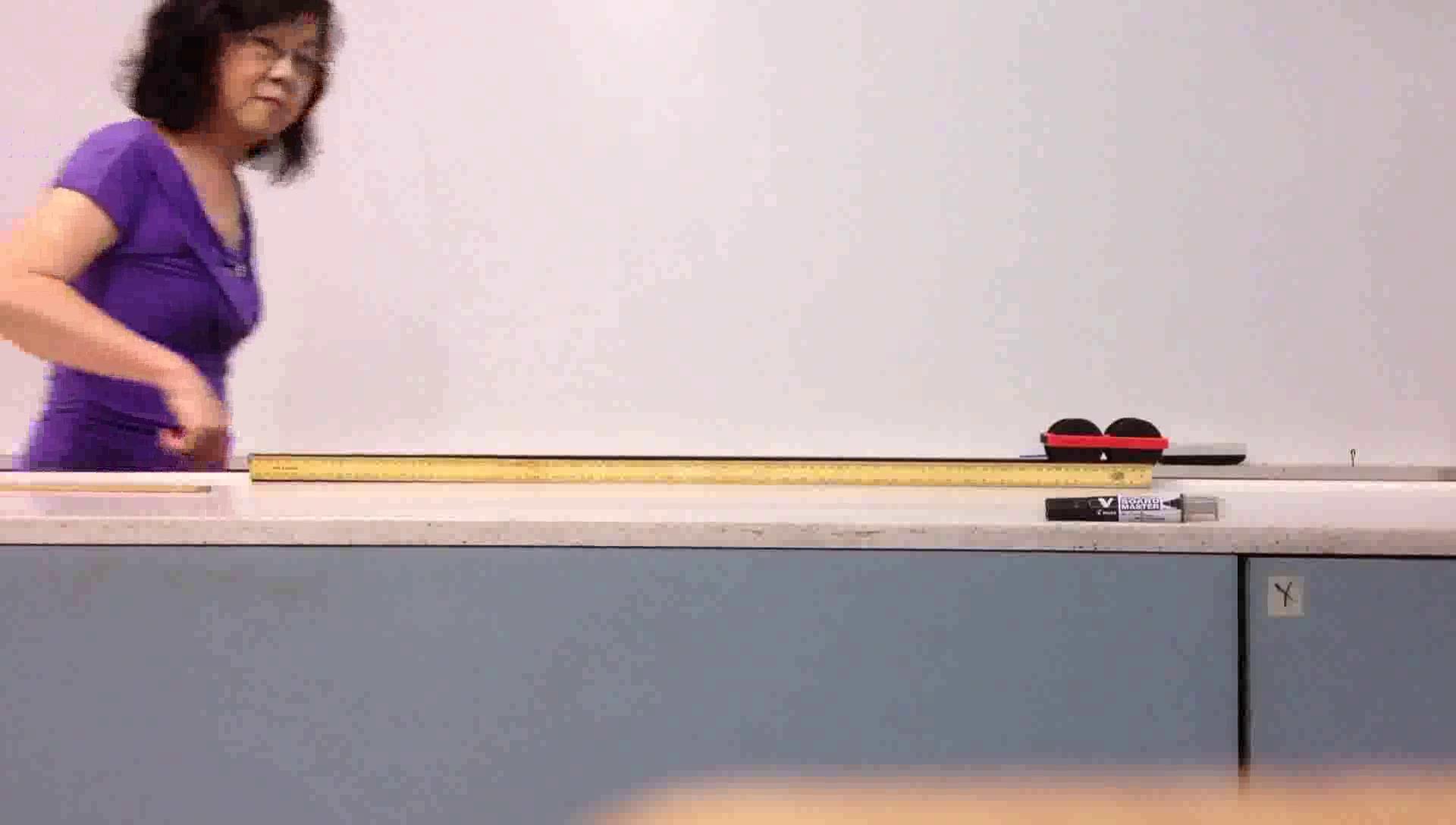
The Tracker Constant Deceleration Cart demonstration is used to study the motion of a cart that is decelerating at a constant rate. This is a classic example in physics used to explore concepts such as acceleration, velocity, distance, and the forces that cause deceleration (like friction or resistance). It is often analyzed with tools like Tracker Video Analysis, which helps visualize and quantify the effects of constant deceleration.

Key Features:

• Uniform Deceleration: The cart moves in such a way that its velocity decreases at a constant rate, ideal for studying uniform motion.
• Data Collection: Tracker can extract data on the cart's velocity, acceleration, and displacement over time.
• Graphing: Automatically generates graphs of velocity versus time, acceleration versus time, and position versus time, which helps students visualize the relationship between these variables in uniformly decelerating motion.
• Modeling: Tracker can model the motion based on physical principles such as Newton's Second Law and the equations of motion for constant acceleration (or deceleration).

Target Audience:

• Physics Students: Essential for understanding concepts like constant acceleration (or deceleration), kinematic equations, and force interactions.
• Teachers/Educators: A powerful teaching tool for illustrating the laws of motion and the effects of forces on an object in a controlled setup.
• Researchers: Useful for performing motion analysis and investigating the dynamics of decelerating objects in experimental physics.

Applications:

• Analyzing the cart's deceleration as a result of friction or air resistance.
• Teaching concepts like Newton's Second Law, kinematics, and energy dissipation.
• Simulating and modeling real-world scenarios involving motion under constant forces.

Study Guide: Tracker Constant Deceleration Cart by Leong Tze Kwang

1. Getting Started

• Installing Tracker: Download the Tracker software from the official website and follow the installation instructions.
• Importing the Video: Load the animation or video of the cart into Tracker by selecting "Open Video." Ensure the video captures the motion clearly for accurate tracking.
• Setting the Reference Frame: Establish a coordinate system and scale for the video by marking fixed reference points. This is essential for correctly interpreting the motion data.

2. Tracking the Cart's Motion

• Manually Tracking: Use Tracker’s manual tracking tool to place a tracker on the cart at each frame. Move through the video frame-by-frame to follow the cart’s motion precisely.
• Automatic Tracking: For simpler movements, use Tracker’s automatic tracking feature to track the cart across frames without having to manually adjust every frame.

3. Analyzing the Cart's Motion

• Velocity and Acceleration: Tracker will calculate the cart’s velocity and acceleration as it moves. Since the cart is undergoing constant deceleration, the acceleration should remain negative and constant.
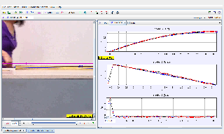
• Position vs. Time: Analyze how the position of the cart changes over time. You should observe the position graph exhibiting a parabolic shape that reflects the cart's slowing motion.
• Velocity vs. Time: Track how the velocity of the cart changes over time. The velocity graph should show a straight line with a negative slope, indicating a constant rate of deceleration.
• Acceleration vs. Time: The acceleration graph should display a horizontal line that remains constant, reflecting the uniform deceleration.

4. Using Kinematic Equations

• Equations of Motion: You can use the equations for uniformly accelerated motion (or decelerated motion in this case) to model and predict the cart’s behavior:
  • v=u+at
  • s=ut+(1/2)at^2
  • v2=u2+2as Where:
  • $v$ is the final velocity,
  • $u$ is the initial velocity,
  • $a$ is the acceleration,
  • $t$ is time,
  • $s$ is displacement.

Note: For the decelerating cart, $a$ will be negative.

5. Creating Graphs and Analyzing Results

• Graphing the Data: Once the tracking data is collected, Tracker can automatically generate several graphs, such as velocity versus time and acceleration versus time. Interpret the graphs to gain insights into the deceleration and other physical properties.
• Energy Analysis: Use Tracker’s tools to explore how the kinetic energy of the cart changes over time as it decelerates, illustrating the work done by the retarding force (e.g., friction or air resistance).

6. Exporting Data

• Exporting to CSV: Export the motion data to a CSV file to conduct further analysis in spreadsheet software like Excel or Google Sheets.
• Creating Reports: Generate and export graphical representations of the data for presentations, reports, or further study.

Frequently Asked Questions (FAQ)

Q1: How do I track the cart’s motion accurately in Tracker?

A1: To track the motion accurately, carefully place the tracker on a fixed point of the cart in each frame, ensuring that the cart’s movement is consistently tracked. If the cart is moving fast, you may need to adjust the tracking speed to capture all details.

Q2: What is the expected graph of the cart’s motion?

A2: For constant deceleration, the position vs. time graph will be parabolic, the velocity vs. time graph will be a straight line with a negative slope, and the acceleration vs. time graph will be a horizontal line at a constant negative value.

Q3: Why is the cart’s acceleration constant?

A3: The cart’s acceleration remains constant because the forces causing the deceleration (like friction or air resistance) do not change as the cart slows down. This is an example of uniform (constant) deceleration.

Q4: How can I measure the force acting on the cart?

A4: You can use Newton’s Second Law of Motion to calculate the force:
F=ma
Where $m$ is the mass of the cart and $a$ is the acceleration (negative for deceleration). If you know the mass and the constant deceleration from your data, you can calculate the retarding force.

Q5: Can I analyze other motions like constant acceleration?

A5: Yes, Tracker can also be used to study motions with constant acceleration (e.g., free fall under gravity) by adjusting the tracking setup and applying appropriate kinematic equations.

Q6: How do I model the decelerating cart in Tracker?

A6: You can use Tracker’s modeling tools to simulate the forces acting on the cart, such as friction. You can also input the known values for mass, initial velocity, and deceleration to model and compare the real video data.

Q7: Can Tracker simulate different types of deceleration?

A7: Yes, Tracker can simulate various types of motion, including constant deceleration and other complex forms, by adjusting parameters such as the forces involved and the object's properties (mass, shape, etc.).