About

Taylor approximations

At the left side of the window one of eight different base functions y = f(x) can be selected by radio buttons. A suitable x range 0 < x < 2a is attributed to each of them.

• sin(x)
• [sin(x)]²
• sin(x²)
• Power function pow (x,7) = x⁷
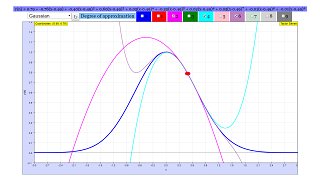
• Gaussian:  exp(-(x-a)²)
• sin(x-a)/(x-a))
• [sin(x-a)/(x-a)]²
• e^x - 2

When opening the simulation, the Gaussian function will be activated and is drawn as a blue curve. The quadratic Taylor approximation around the origin is shown in magenta.

At the top of the window there are 9 radio buttons to select a Taylor approximation (expansion) around a model point x_o, of index 0 (constant value y₀) to 9 (considering up to the 9th derivative in x_0, y₀ ). The selected approximations is drawn in the color of the radio buttons .

The model point x0, y0 is shown as a red dot. It can be drawn with the mouse to calculate the expansion around an arbitrary model point.

Reset Dot returns the model point to its default position.

The first number field at the left shows the value of the function y₀ in the model point x₀, y₀.

The other number fields show the factors of the power functions ( x-x₀ ) ⁿ in the Taylor series, as

f5 = y⁽⁵⁾/5!

Very small numbers at high index may indicate numerical artifacts.

Taylor series

This simulation calculates the Taylor series of a function

y = f(x)

in the vicinity of a model point x_0, y₀

y = f(x₀) + f ´(x₀)(x - x₀)/1! + f´´(x0)(x - x₀)²/2!+... + f⁽ⁿ⁾(x₀)(x - x₀)ⁿ/n!...

n! = 1∙2∙3∙4...∙ n:  n faculty

The first member of the series is an approximation within the interval by the value in the model point:  y ≈ f(x₀). This is commonly called the zeroth approximation.

The first approximation considers the first derivative, and is the tangent to the curve at the model point. It is also called the linear approximation and is already quite useful for small intervals.

y ≈ f(x₀) + f ´(x₀)(x - x₀)/1! = f(x₀) + f´(x₀)(x - x₀)

The second or quadratic approximation adds a parabola of second order, considering also the curvature in the model point.

y ≈ f(x₀) + f ´(x₀)(x - x₀)/1! + f´´(x0)(x - x₀)²/2

(One should realize that the resulting polynom of second order is not identical to the parabola used in the Kepler algorithm of integration:  The Kepler parabola cuts the curve in three points, while the Taylor polynom touches it in one. Both approximations converge with decreasing interval width of integration).

The higher order approximations are polynomials of increasing order, which approach the function well over wider and wider intervals (for "well behaved" functions, which our examples are).

For the example of a 7th power parabola the 7th Taylor approximation is identical to the function itself, as all higher derivatives are 0. (the very small deviations from 0 seen in the number fields for f8 and f9 are residual calculation errors).

(x - 0)⁷ = y0 + f1(x - x0) + f2 (x - x0)² + f3(x - x0)³ + f4(x - x0)⁴ + f5(x - x0)⁵

+ f6(x - x0)⁶ + f7(x - x0)⁷

The identity demonstrates that the original parabola x⁷can be interpreted as a Taylor expansion around x = 0. Indeed, as one draws the dot to x = 0, all factors in the number fields become zero except f7, which will be 1.

Calculation of the derivatives

With h − the difference between consecutive x values − sufficiently small, the first derivative (differential quotient) is approximated by the difference quotient:

y⁽¹⁾(x) = (1/2h) [y(x+h) - y(x-h)]

The second derivative is approximated as the difference quotient of the first difference quotient:

y⁽²⁾(x)= (1/2h) [y⁽¹⁾(x+h) - y⁽¹⁾(x-h)] = (1/2h)² [y(x+2h) - 2y(x) + y(x-1h)]

This algorithm can be continued, leading to the code lines shown below for the base function a[0] and its derivatives up to the 9th order a[9].

For the predefined functions most approximations do not differ visibly from the analytical derivatives, with the interval h being 1/1000 of the total range.

For still higher derivatives the limits of the accuracy of the approximation and also of the computing accuracy are stressed, and noise appears.

Code for calculating the derivatives: With s = 1/(2h)

a0=y0;

a1[j]=Math.pow(s,1)*(y2[1][j]-y1[1][j]);

a2[j]=Math.pow(s,2)*(y2[2][j]-2*y2[0][j]+y1[2][j]);

a3[j]=Math.pow(s,3)*(y2[3][j]-3*y2[1][j]+3*y1[1][j]-y1[3][j]);

a4[j]=Math.pow(s,4)*(y2[4][j]-4*y2[2][j]+6*y2[0][j]-4*y1[2][j]+y1[4][j]);

a5[j]=Math.pow(s,5)*(y2[5][j]-5*y2[3][j]+10*y2[1][j]-10*y1[1][j]+5*y1[3][j]-y1[5][j]);

a6[j]=Math.pow(s,6)*(y2[6][j]-6*y2[4][j]+15*y2[2][j]-20*y2[0][j]+15*y1[2][j]-6*y1[4][j]+y1[6][j]);

a7[j]=Math.pow(s,7)*(y2[7][j]-7*y2[5][j]+21*y2[3][j]-35*y2[1][j]+35*y1[1][j]-21*y1[3][j]+7*y1[5][j]-y1[7][j]);

a8[j]=Math.pow(s,8)*(y2[8][j]-8*y2[6][j]+28*y2[4][j]-56*y2[2][j]+70*y2[0][j]-56*y1[2][j]+28*y1[4][j]-8*y1[6][j]+y1[8][j]);

a9[j]=Math.pow(s,9)*(y2[9][j]-9*y2[7][j]+36*y2[5][j]-84*y2[3][j]+126*y2[1][j]-126*y1[1][j]+84*y1[3][j]-36*y1[5][j]+9*y1[7][j]-y1[9][j]);

Code for calculating the Taylor approximations

T0[j]=a0;

T1[j]=T0[j]+Math.pow(x-x0,1)*a1/(1);

T2[j]=T1[j]+Math.pow(x-x0,2)*a2/(1*2);

T3[j]=T2[j]+Math.pow(x-x0,3)*a3/(1*2*3);

T4[j]=T3[j]+Math.pow(x-x0,4)*a4/(1*2*3*4);

T5[j]=T4[j]+Math.pow(x-x0,5)*a5/(1*2*3*4*5);

T6[j]=T5[j]+Math.pow(x-x0,6)*a6/(1*2*3*4*5*6);

T7[j]=T6[j]+Math.pow(x-x0,7)*a7/(1*2*3*4*5*6*7);

T8[j]=T7[j]+Math.pow(x-x0,8)*a8/(1*2*3*4*5*6*7*8);

T9[j]=T8[j]+Math.pow(x-x0,9)*a9/(1*2*3*4*5*6*7*8*9);

The integers in the formulas of the derivatives follow simple generation rules; thus the series can be easily generated or continued.

E1:

• The zero order approximation assumes that the value in the model point is true for the whole interval.
• The first order considers the local steepness of the function curve.
• The second derivative considers the local change in steepness = curvature.
• The third derivative considers the local change in curvature =  ?
• The fourth derivative considers the local change in the change of curvature = ??
• ...and so on.

Try to understand what the higher derivatives mean, as applied to the Taylor approximation of a function.

E2:  Do that for the sine function. Why does the 4th approximation not look like the base function itself? (the 4th derivative alone is identical to it).

E3:  Go through the approximations of the power function:  What type of polynom is each one? (Write them down, using the factors in the number fields). Check that 7th to 9th are identical (tiny differences recognizable are calculation errors). Compare the 7th order polynoms around different model points and argue their identity. Look at the one for x₀ = 0.

E4: Experiment with all base functions. Consider why and when a linear approximation, which is easy to handle analytically, is good enough. Take a look at the sequence factors.

This simulation was created in May 2010 by Dieter Roess

This simulation is part of

“Learning and Teaching Mathematics using Simulations

– Plus 2000 Examples from Physics”

ISBN 978-3-11-025005-3, Walter de Gruyter GmbH & Co. KG

 

Translations

Code	Language		Translator	Run

Credits

Dieter Roess - WEH- Foundation; Tan Wei Chiong; Loo Kang Wee

Overview:

This document provides a briefing on a JavaScript simulation applet designed to illustrate the concept of Taylor series approximations of functions. The applet, part of the "Open Educational Resources / Open Source Physics @ Singapore" project, allows users to interactively explore how Taylor polynomials of increasing degrees can approximate various base functions around a chosen model point.

Main Themes and Important Ideas:

1. Taylor Series Approximation: The core concept is the approximation of a function y = f(x) around a specific point x0, y0 using a sum of terms calculated from the function's derivatives at that point. The general formula for the Taylor series is provided:
2. y = f(x0) + f ´(x0)(x - x0)/1! + f´´(x0)(x - x0)2/2!+... + f(n)(x0)(x - x0)n /n!...
3. Interactive Simulation: The applet offers a visual and interactive way to understand Taylor series. Key features include:

• Selectable Base Functions: Users can choose from eight different predefined functions using radio buttons, each with a defined x-range. Examples include sin(x), [sin(x)]^2, x^7, exp(-(x-a)^2), etc.
• Adjustable Order of Approximation: Nine radio buttons allow users to select Taylor approximations from the 0th order (constant) up to the 9th order (using the 9th derivative). Each selected approximation is drawn in a distinct color.
• Movable Model Point: A red dot represents the model point (x0, y0) around which the Taylor series is expanded. Users can drag this point with the mouse to observe how the Taylor approximations change.
• Numerical Display of Coefficients: Number fields display the value of the function at the model point (y0) and the factors of the power terms (x - x0)^n in the Taylor series. The formula for these factors is given as f5 = y(5)/5!, highlighting the relationship between the coefficients and the derivatives.

1. Understanding Orders of Approximation: The simulation helps visualize the meaning of different order Taylor approximations:

• Zero-order approximation: y ≈ f(x0) - A horizontal line representing the function's value at the model point.
• First-order (linear) approximation: y ≈ f(x0) + f ´(x0)(x - x0) - The tangent line to the curve at the model point, representing the local steepness. The source notes this is "already quite useful for small intervals."
• Second-order (quadratic) approximation: y ≈ f(x0) + f ´(x0)(x - x0)/1! + f´´(x0)(x - x0)^2 /2! - Adds a parabola, considering the curvature at the model point. The text distinguishes this from Kepler's parabola used in integration.
• Higher-order approximations: Polynomials of increasing degree that provide better approximations over wider intervals for well-behaved functions. For example, for a 7th power function, the 7th Taylor approximation becomes identical to the original function.

1. Numerical Calculation of Derivatives: The applet uses a numerical method to approximate the derivatives of the selected functions. It employs the difference quotient method:
2. *y(1) (x) = (1/2h) [y(x+h) - y(x-h)] *y(2)(x)= (1/2h) [y(1)(x+h) - y(1)(x-h)] = (1/2h)^2 [y(x+2h) - 2y(x) + y(x-1h)] The simulation uses a small value for h (1/1000 of the total range) for these approximations. The text mentions that "For still higher derivatives the limits of the accuracy of the approximation and also of the computing accuracy are stressed, and noise appears."
3. Code Implementation: The source provides snippets of the JavaScript code used to calculate the derivatives (up to the 9th order) and the Taylor approximations (T0 to T9). These code examples illustrate the recursive nature of the Taylor series calculation, where each higher-order approximation builds upon the previous one.
4. Experiments and Learning Goals: The "Experiments" section suggests activities for users to explore the properties of Taylor approximations, such as the meaning of higher derivatives (E1), applying the concept to the sine function (E2), analyzing the Taylor series of a power function (E3), and considering the utility of linear approximations (E4). The "Sample Learning Goals" and "For Teachers" sections further emphasize the educational purpose of the simulation in understanding polynomial approximations of functions.
5. Context and Authorship: The simulation was created by Dieter Roess in May 2010 and is part of a larger project focused on using simulations for learning and teaching mathematics and physics. Credits are also given to Tan Wei Chiong and Loo Kang Wee.

Key Quotes:

• "This simulation calculates the Taylor series of a function y = f(x) in the vicinity of a model point x0, y0"
• "The first approximation considers the first derivative, and is the tangent to the curve at the model point. It is also called the linear approximation and is already quite useful for small intervals."
• "The second or quadratic approximation adds a parabola of second order, considering also the curvature in the model point."
• "For the example of a 7th power parabola the 7th Taylor approximation is identical to the function itself, as all higher derivatives are 0."
• "For the predefined functions most approximations do not differ visibly from the analytical derivatives, with the interval h being 1/1000 of the total range."
• "The Taylor Series is a generalised polynomial approximation to a function, centered around x = a, for any real number a."

Conclusion:

The Taylor Series Approximation JavaScript Simulation Applet provides a valuable interactive tool for understanding the fundamental concept of approximating functions using Taylor series. By allowing users to select different functions, adjust the order of approximation, and move the expansion point, the applet fosters intuitive learning about the relationship between a function, its derivatives, and its polynomial approximations. The inclusion of code snippets and suggested experiments further enhances its educational value for students and teachers of mathematics and physics.

 

Taylor Series Approximation Study Guide

Key Concepts

• Taylor Series: An infinite sum of terms expressed in terms of the function's derivatives at a single point. It provides a way to approximate a function as a polynomial.
• Taylor Approximation: A finite number of terms from the Taylor series, used to approximate the value of a function near a specific point. The more terms included, the better the approximation generally becomes within a certain radius of convergence.
• Model Point (x₀, y₀): The point around which the Taylor series is expanded. The derivatives of the function are evaluated at x₀, and y₀ = f(x₀). This point can be manipulated in the simulation.
• Order of Approximation: The highest derivative included in the Taylor approximation. A zero-order approximation only considers the function value at x₀, a first-order (linear) approximation includes the first derivative, a second-order (quadratic) approximation includes the second derivative, and so on.
• Derivatives: The rate of change of a function with respect to its variable. The first derivative represents the slope of the tangent line, the second derivative represents the curvature, the third represents the rate of change of curvature, and higher derivatives represent further rates of change.
• Factorial (n!): The product of all positive integers up to n (e.g., 5! = 5 × 4 × 3 × 2 × 1 = 120). Factorials appear in the denominator of the terms in the Taylor series formula.
• Linear Approximation: The first-order Taylor approximation, which uses the tangent line to approximate the function near the model point.
• Quadratic Approximation: The second-order Taylor approximation, which uses a parabola to approximate the function near the model point, taking into account the function's curvature.
• Numerical Artifacts: Small errors in calculations that appear, especially with higher-order approximations, due to the limitations of computer precision.

Quiz

1. What is the fundamental idea behind using a Taylor series to approximate a function? Explain in 2-3 sentences.
2. Describe the role of the "model point" in the context of Taylor series approximation. How does changing this point affect the approximation?
3. What does the order of a Taylor approximation signify? Explain the difference between a zero-order and a first-order approximation.
4. How is the first derivative of a function related to its first-order Taylor approximation? What does this approximation represent geometrically?
5. What information about a function does the second derivative provide, and how is this incorporated into the second-order Taylor approximation?
6. According to the simulation's description, what happens to the accuracy of the Taylor approximation as more terms (higher derivatives) are included for "well behaved" functions?
7. Why does the simulation indicate that for a 7th power parabola, the 7th Taylor approximation is identical to the function itself? What does this imply about the higher derivatives of such a function?
8. Explain how the simulation calculates the first and second derivatives numerically. What parameter 'h' is crucial in this calculation?
9. What are some potential limitations or challenges encountered when calculating very high-order Taylor approximations, as suggested by the text?
10. How does the Taylor polynomial in the simulation differ from the parabola used in Kepler's algorithm for integration, according to the description?

Quiz Answer Key

1. The fundamental idea is to represent a complex function locally as a simpler polynomial. The Taylor series achieves this by matching the function's value and the values of its derivatives at a specific point (the model point) with those of the polynomial.
2. The model point (x₀, y₀) is the center around which the Taylor series is constructed. The approximation is generally most accurate near this point, and shifting the model point results in a different Taylor series expansion and thus a different polynomial approximation.
3. The order of approximation indicates the highest derivative of the function included in the polynomial. A zero-order approximation is just the function value at the model point (a constant), while a first-order approximation (linear) includes the first derivative and represents the tangent line at that point.
4. The first derivative, evaluated at the model point, determines the slope of the first-order Taylor approximation (the tangent line). This linear approximation represents the best linear fit to the function in the immediate vicinity of the model point.
5. The second derivative provides information about the function's curvature (how the slope is changing). The second-order Taylor approximation (quadratic) incorporates this curvature by adding a term involving the second derivative, resulting in a parabolic approximation that better fits the function's shape.
6. For "well behaved" functions, including more terms (higher derivatives) in the Taylor approximation generally leads to a more accurate approximation over a wider interval around the model point, as the polynomial better captures the function's nuances.
7. For a 7th power parabola, all derivatives higher than the 7th are zero. Therefore, the Taylor series expansion beyond the 7th order adds only zero terms, making the 7th Taylor polynomial exactly equal to the original 7th power function.
8. The simulation uses finite difference quotients to approximate the derivatives. The first derivative is approximated using values at x+h and x-h, and the second derivative is approximated using values at x+2h, x, and x-h, where 'h' is a sufficiently small difference between consecutive x values.
9. Calculating very high-order Taylor approximations can lead to limitations in accuracy due to the approximation method itself and the finite precision of computer calculations, resulting in the appearance of "noise" or numerical artifacts.
10. The Taylor polynomial touches the curve at only one point (the model point) and matches its derivatives there, while the Kepler parabola cuts the curve at three points. Both are approximations that improve with a decreasing interval width.

Essay Format Questions

1. Discuss the significance of Taylor series in approximating functions, particularly in contexts where analytical solutions are difficult or unavailable. How does the order of the approximation relate to its accuracy and range of validity?
2. Explain the concept of the model point in Taylor series approximation and analyze how its placement affects the resulting polynomial approximation. Consider different types of functions and the strategic choices one might make for the model point.
3. The simulation demonstrates Taylor approximations for various base functions. Choose two contrasting functions (e.g., sin(x) and x⁷) and analyze how their Taylor series approximations of increasing order behave differently. What properties of the original functions explain these differences?
4. The text mentions the linear and quadratic approximations as particularly useful. Discuss the practical applications of these lower-order Taylor approximations in science, engineering, or mathematics, providing specific examples where they offer valuable insights or simplifications.
5. Critically evaluate the limitations of Taylor series approximations, considering factors such as the behavior of the function, the distance from the model point, and the potential for numerical errors in high-order approximations. Under what conditions might a Taylor series approximation be unreliable or impractical?

Glossary of Key Terms

• Base Function: The original function, y = f(x), that is being approximated by the Taylor series in the simulation.
• Convergence: The property of an infinite series where the sum of its terms approaches a finite limit as the number of terms increases. Taylor series for some functions converge to the function's value within a certain interval.
• Derivative Quotient (Difference Quotient): An approximation of the derivative of a function at a point using the values of the function at nearby points. Used in numerical differentiation.
• Embed: To integrate or insert external content, like the simulation applet, into a webpage.
• Expansion (Taylor Expansion): Another term for the Taylor series, emphasizing the process of expressing a function as an infinite sum.
• Index: A numerical label used to identify the position or order of a term, such as the order of the derivative in the Taylor series.
• Polynomial: An expression consisting of variables and coefficients, involving only the operations of addition, subtraction, multiplication, and non-negative integer exponents of variables. Taylor approximations are polynomials.
• Radio Buttons: Graphical user interface elements that allow the user to select only one option from a set of choices. Used in the simulation to select the base function and the order of the Taylor approximation.
• Vicinity: The region or interval around a specific point. Taylor series provide good approximations of a function in the vicinity of the model point.

Sample Learning Goals

[text]

For Teachers

The Taylor Series is a generalised polynomial approximation to a function, centered around x = a, for any real number a.

In this simulation, you can choose a function to approximate with the Taylor Series from the combo box provided. However, this is technically not a series, as the terms do not go indefinitely.

Beside the combo box for selecting the function, there is a set of 10 checkboxes, each of them corresponding to a certain degree of approximation. The degree of the polynomial approximation is shown by the number beside the checkbox. When each box is checked, the graph of the polynomial corresponding to the degree denoted by the checkbox is made visible; unchecking it will make it invisible.

The available functions are as follows:
- Gaussian: y = e^-(x^2)
- y = sin(x)
- y = sin(x)^2
- y = sin(x)/x
- sin(x)/x Quadratic: y = [sin(x)/x]^2
- y = x^7
- y = e^x

At the top of the simulation, the full 9th degree polynomial approximation for the function at the point denoted by the square in the graph is shown, and will automatically change when the point is moved. Likewise, the graphs of the different polynomial approximations will also adjust accordingly.

Research

[text]

Video

[text]

 Version:

1. http://weelookang.blogspot.sg/2016/02/vector-addition-b-c-model-with.html improved version with joseph chua's inputs
2. http://weelookang.blogspot.sg/2014/10/vector-addition-model.html original simulation by lookang

Other Resources

[text]

What is a Taylor series approximation?

A Taylor series approximation is a way to represent a function as a sum of terms calculated from the function's derivatives at a single point. It provides a polynomial approximation of a function around a specific point, with the accuracy of the approximation generally improving as more terms (higher-order derivatives) are included in the series.

How does the provided simulation demonstrate Taylor series approximations?

The JavaScript simulation allows users to select from eight different base functions and then explore Taylor series approximations of these functions around a movable model point (x0, y0). By choosing different degrees of approximation (from 0th to 9th derivative), users can visually compare how well the polynomial approximation matches the original function curve. The simulation also displays the coefficients of the Taylor series terms, illustrating the contribution of each derivative.

What is the significance of the "model point" (x0, y0) in a Taylor series?

The model point (x0, y0) is the center around which the Taylor series expansion is calculated. The Taylor series expresses the value of the function at points near x0 using the function's value and the values of its derivatives at x0. Changing the model point will result in a different Taylor series representation of the same function, as the derivatives are evaluated at the new center.

How do different orders of Taylor series approximations compare?

Lower-order approximations provide a simpler representation of the function. The zero-order approximation is just the function's value at the model point (a horizontal line). The first-order (linear) approximation is the tangent line to the curve at that point, considering the function's slope. Higher-order approximations (quadratic, cubic, etc.) incorporate higher derivatives, adding terms that account for the function's curvature, rate of change of curvature, and so on. Generally, higher-order approximations are more accurate over a wider interval around the model point for "well-behaved" functions.

Why might a lower-order (e.g., linear) Taylor approximation be useful?

Lower-order Taylor approximations, particularly the linear approximation, are often useful because they are simpler to work with analytically. They can provide a good estimate of a function's behavior in a small interval around the model point. This simplicity is valuable in situations where a precise representation over a large interval is not required, or when the function itself is complex and difficult to manipulate directly.

How are the derivatives of the function calculated in this simulation?

The simulation uses a numerical method based on the difference quotient to approximate the derivatives of the selected base functions. For the first derivative, it uses a central difference approximation: y'(x) ≈ (1/2h) [y(x+h) - y(x-h)], where 'h' is a small difference in x values. Higher-order derivatives are approximated by applying the difference quotient to the lower-order derivative approximations iteratively. The code snippets provided in the description illustrate the formulas used for derivatives up to the 9th order.

For a 7th power function (x^7), why does the 7th Taylor approximation match the function exactly?

For a polynomial of degree 'n', all derivatives of order higher than 'n' are zero. In the case of x^7, all derivatives of order 8 and higher will be zero. Therefore, the Taylor series expansion of x^7 around any point will have a finite number of non-zero terms, up to the term involving the 7th derivative. When the Taylor series is expanded to the 7th order, it includes all the non-zero terms and perfectly reconstructs the original polynomial function.

What are some potential limitations or considerations when using Taylor series approximations, as suggested by the simulation?

The simulation highlights that for very high-order derivatives, "numerical artifacts" or "noise" may appear. This indicates that the accuracy of the numerical derivative calculation can be limited by the precision of the computing system. Additionally, while higher-order approximations generally improve accuracy, they are still approximations and may not perfectly match the function over an infinite interval, especially for functions that are not "well-behaved" (e.g., those with singularities or discontinuities). The simulation also notes that for the sine function, the 4th approximation might not look exactly like the base function, reminding users that a high-order derivative being similar to the original function doesn't automatically mean a low-order Taylor series using that derivative will be a perfect match.