
.png
)


About
Riemann integral
In two dimensions the Rieman integral determines the area between the x axis and the function y = f(x) in an interval x1 < x < x2 by nesting it between two approximative sums. Both are constructed by a series of rectangles with intervals along the x axis. For the upper sum the approximative value of y in each interval is equal to the largest value in the interval (its supremum); for the lower sum it is equal to the smalles value (infimum). The Riemann integral exists, when both sums converge with decreasing interval width, and when they converge to the same limit.
The definition is not identical to the classical rectangle algorithm, where the value of the function is equal to the value at the beginning of the interval (more generally: always at the same point in the interval). For "well behaved" functions there will be no difference in results, yet the Riemann definition is more generally applicable.
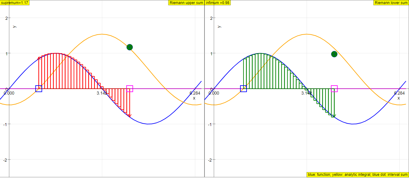
The approximative calculation of the Riemann integral is shown for the example of a sine function (blue). Its definite integral is to be calculated in the range x2 - x1. The initial value x1 is defined by a slider, the end point x2 by drawing the red point with the mouse. The yellow curve is the analytic solution cos x - cos x1.
The number of intervals (n - 1) is defined by slider n. Reset defines 1 < x < 4 and n = 10 (9 intervals) .
The left window shows in red the approximation by the supremum series, with the blue point as the sum; the function always lies below the rectangle. The right window shows the approximation by the infimum series; the function always lies above the rectangle.
Correspondingly the upper sum of the rectangles is always higher than the analytic integral, while the lower sum is always lower - for finite interval widths. With decreasing interval widths both converge to the same value, the Riemann integral.
E1: Start with the default setting: x1 = 1; x2 = 4; n = 10.
Verify that both graphs really limit the intervals in the y direction by the highest, respectively the lowest value in the interval (observe the sign of the function itself!). Consider the systematic deviation of the sum from the analytic solution.
E2: Compare the construction with the classical rectangle (step) algorithm.
E4: Increase n and observe the process of convergence to the limit value as the interval width decreases.
E4: Draw the end point at a large number for n and observe how the intervals limit lines "paint" the area under the curve. You will not visibly recognize a difference between sum and integral.
E5: Change the initial point with the slider. Draw the end point beyond the initial point and control if the result is still correct.
Translations
| Code | Language | Translator | Run | |
|---|---|---|---|---|
 |
||||
Credits
 Dieter Roess - WEH-Foundation; Fremont Teng; Loo Kang Wee
Physics @ Singapore
1. Overview:
This document provides a briefing on the Riemann Integral JavaScript Simulation Applet HTML5, an interactive tool available on the Open Educational Resources / Open Source Physics @ Singapore website. The applet is designed to visually demonstrate the concept of the Riemann integral and its calculation through upper and lower sums. It aims to enhance the learning and teaching of calculus, specifically the definite integral.
2. Main Themes and Important Ideas:
- Definition of the Riemann Integral: The applet focuses on illustrating the formal definition of the Riemann integral, which involves approximating the area under a curve by nesting it between two sums: the upper sum (using the supremum of the function in each interval) and the lower sum (using the infimum).
- "In two dimensions the Rieman integral determines the area between the x axis and the function y = f(x) in an interval x1 < x < x2by nesting it between two approximative sums. Both are constructed by a series of rectangles with intervals along the x axis. For the upper sum the approximative value of y in each interval is equal to the largest value in the interval (its supremum ); for the lower sum it is equal to the smalles value (infimum ). The Riemann integral exists, when both sums converge with decreasing interval width, and when they converge to the same limit."
- Comparison with the Rectangle Algorithm: The source explicitly differentiates the Riemann integral definition from the simpler "rectangle algorithm" (where the function's value is taken at a specific point in the interval, often the beginning). While results may be the same for "well behaved" functions, the Riemann definition is presented as more generally applicable.
- "The definition is not identical to the classical rectangle algorithm , where the value of the function is equal to the value at the beginning of the interval (more generally: always at the same point in the interval). For 'well behaved' functions there will be no difference in results, yet the Riemann definition is more generally applicable."
- Visual Approximation: The applet provides a visual representation of the upper and lower sums using red rectangles (supremum) and implicitly through the bounded blue point sum and the function's position relative to these rectangles. The example of a sine function (blue curve) is used, with the analytic solution displayed as a yellow curve.
- "The left window shows in red the approximation by the supremum series, with the blue point as the sum; the function always lies below the rectangle. The right window shows the approximation by the infimum series; the function always lies above the rectangle."
- "Correspondingly the upper sum of the rectangles is always higher than the analytic integral, while the lower sum is always lower - for finite interval widths. With decreasing interval widths both converge to the same value, the Riemann integral."
- Interactive Exploration: The applet offers several interactive features to allow users to explore the Riemann integral concept:
- Sliders: An "n" slider controls the number of intervals used for the approximation, allowing users to observe the effect of decreasing interval width on the convergence of the upper and lower sums to the Riemann integral. An "x1" slider defines the starting point of the integration interval.
- Draggable Point: A red point can be dragged with the mouse to set the end point (x2) of the integration interval.
- Reset Button: Resets the simulation to a default setting (x1 = 1, x2 = 4, n = 10).
- Full Screen Toggle: Allows for an expanded view of the simulation.
- Convergence: A key idea highlighted is the convergence of both the upper and lower sums to the same limit as the number of intervals increases (and the interval width decreases). This convergence is the condition for the existence of the Riemann integral.
- "With decreasing interval widths both converge to the same value, the Riemann integral."
- Experiment E4 encourages users to "Increase n and observe the process of convergence to the limit value as the interval width decreases."
- Experiment E4 also notes that with a large number of intervals, the difference between the sum and the integral becomes visually indistinguishable.
- Systematic Deviation: Experiment E1 encourages users to observe the "systematic deviation of the sum from the analytic solution" for finite interval widths, reinforcing the idea that the Riemann sum is an approximation that improves with more intervals.
- Applicability: The applet is designed as a learning tool for calculus, categorized under "Learning and Teaching Mathematics using Simulations."
3. Instructions for Use (Key Features):
- N Slider: Controls the number of rectangles (intervals) used in the approximation.
- Draggable Box (Red Point): Sets the end point (x2) of the integration interval.
- Reset Button: Returns the simulation to its initial state.
- Toggling Full Screen: Enlarges the applet view.
4. Experiments Suggested:
The "Experiments" section provides guided activities for users to engage with the simulation and deepen their understanding:
- E1: Observe the upper and lower bounds provided by the supremum and infimum rectangles and the deviation from the analytic solution at the default settings.
- E2: Compare the Riemann integral construction with the classical rectangle algorithm (though this is not directly visualized, the user can conceptually compare the upper/lower bound approach to a single-point evaluation).
- E4: Increase the number of intervals (n) to witness the convergence of the sums to the integral.
- E5: Change the starting point (x1) and the direction of integration to test the applet's correctness.
5. Context and Related Resources:
The applet is part of a larger collection of "Open Educational Resources / Open Source Physics @ Singapore," which includes numerous other JavaScript simulations for various topics in mathematics and physics. The page provides links to other related applets, such as "Definite Integral JavaScript Simulation Applet HTML5" and "Integral: Algorithms of Numerical Approximation JavaScript Simulation Applet HTML5," suggesting a broader focus on integral calculus concepts within this resource. The extensive list of other simulations demonstrates the breadth of topics covered by this platform.
6. Credits and Licensing:
The applet is credited to Dieter Roess, Fremont Teng, and Loo Kang Wee. The content is licensed under the Creative Commons Attribution-Share Alike 4.0 Singapore License, promoting open access and sharing. Commercial use of the underlying EasyJavaScriptSimulations Library requires a separate license and contact with the developers.
7. Conclusion:
The Riemann Integral JavaScript Simulation Applet HTML5 is a valuable interactive tool for learning and teaching the fundamental concept of the Riemann integral. By visually demonstrating the upper and lower sum approximations and allowing for user experimentation with parameters like the number of intervals and the integration range, it provides a more intuitive understanding of this crucial calculus concept and its formal definition. The comparison with the rectangle algorithm and the focus on convergence further enhance its educational value.
Key Concepts
- Riemann Integral: A method to determine the area between the x-axis and a function y = f(x) over a given interval by approximating it with upper and lower sums.
- Upper Sum: An approximation of the area using rectangles where the height of each rectangle is the supremum (largest value) of the function within that interval. The function lies below these rectangles.
- Lower Sum: An approximation of the area using rectangles where the height of each rectangle is the infimum (smallest value) of the function within that interval. The function lies above these rectangles.
- Convergence: The property of the upper and lower sums approaching the same limit as the width of the intervals of the rectangles decreases. The Riemann integral exists if and only if both sums converge to the same value.
- Rectangle Algorithm (Step Algorithm): A simpler approximation method where the height of each rectangle is determined by the function's value at a specific point in the interval, often the beginning. While it yields the same result for "well-behaved" functions, the Riemann definition is more general.
- Analytic Solution: The exact solution to the definite integral, often found using the fundamental theorem of calculus (e.g., the yellow curve cos x - cos x1 in the simulation).
- Interval Width: The width of each rectangle along the x-axis. Decreasing the interval width (increasing the number of intervals) generally leads to a more accurate approximation of the Riemann integral.
- Supremum: The least upper bound of a set of values within an interval.
- Infimum: The greatest lower bound of a set of values within an interval.
- Slider (n): A control element in the simulation that allows the user to adjust the number of intervals used in the approximation.
- Draggable Box: A feature in the simulation that allows the user to define the endpoints of the interval (x1 and x2) over which the Riemann integral is calculated.
- Reset Button: A function in the simulation that returns the settings to a default state (e.g., x1 = 1, x2 = 4, n = 10).
Quiz
- Explain in your own words how the Riemann integral approximates the area under a curve. What are the two types of sums used in this approximation?
- What is the key difference between the definition of the Riemann integral and the classical rectangle algorithm for approximating the area under a curve? Why is the Riemann definition considered more generally applicable?
- Describe the role of the upper sum and the lower sum in the definition of the Riemann integral. How are the heights of the rectangles determined for each of these sums within a given interval?
- What does it mean for the upper and lower sums to "converge" in the context of the Riemann integral? When does the Riemann integral exist based on this convergence?
- In the provided JavaScript simulation, how can you adjust the interval over which the Riemann integral is calculated? What visual elements represent the upper and lower sums?
- Explain what the "analytic solution" represents in the context of the simulation. How does it relate to the approximations provided by the upper and lower sums?
- Describe what happens to the upper and lower sums as you increase the value of 'n' using the slider in the simulation. Why does this change occur?
- What is the significance of the supremum and infimum in the formal definition of the Riemann integral? How do these concepts relate to the construction of the upper and lower sums?
- Based on Experiment E1, what systematic deviation might you observe between the upper and lower sums and the analytic solution for a finite number of intervals? Why does this deviation occur?
- How does the simulation demonstrate the idea that as the interval width decreases, the difference between the upper sum, lower sum, and the Riemann integral becomes less noticeable?
Quiz Answer Key
- The Riemann integral approximates the area under a curve by dividing the interval into smaller subintervals and constructing rectangles on each subinterval. The height of these rectangles is determined by the function's values within that subinterval. The two types of sums are the upper sum (using the maximum value in each subinterval) and the lower sum (using the minimum value).
- The Riemann integral's definition uses the supremum and infimum of the function within each interval to determine the rectangle heights, whereas the classical rectangle algorithm uses the function's value at a specific point (like the beginning) of the interval. The Riemann definition is more generally applicable because it works for a broader range of functions, even those with discontinuities within the interval.
- The upper sum provides an overestimate of the area because the height of each rectangle is the supremum (largest y-value) of the function in that interval, ensuring the rectangle encloses the function in that section. Conversely, the lower sum gives an underestimate as the rectangle's height is the infimum (smallest y-value), placing the rectangle entirely below the function in that interval.
- Convergence means that as the width of the subintervals approaches zero (the number of intervals approaches infinity), both the upper and lower sums get closer and closer to a single, shared value. The Riemann integral exists if and only if these two sums converge to the same finite limit.
- In the simulation, the interval is adjusted by dragging the red point with the mouse, which defines the endpoint x2, while the slider sets the initial point x1. The left window visually represents the upper sum (red rectangles), and the right window shows the lower sum (red rectangles).
- The analytic solution is the exact value of the definite integral of the function over the chosen interval, represented by the yellow curve in the simulation. It is the theoretical area under the curve, and the upper and lower sums are approximations that should converge to this value as the number of intervals increases.
- As you increase the value of 'n', the number of intervals increases, and the width of each interval decreases. This leads to the upper sum decreasing and the lower sum increasing, as the rectangles become a better fit to the shape of the curve, resulting in a more accurate approximation of the true area.
- The supremum (least upper bound) and infimum (greatest lower bound) are crucial for the formal definition of the Riemann integral because they provide a rigorous way to define the "highest" and "lowest" values of the function within each subinterval, even for functions that may not attain a clear maximum or minimum value.
- For a finite number of intervals, the upper sum will typically be greater than or equal to the analytic solution, while the lower sum will be less than or equal to the analytic solution. This is because the upper sum's rectangles tend to include area above the curve, and the lower sum's rectangles tend to exclude area under the curve.
- The simulation visually demonstrates convergence by showing that as 'n' increases and the interval width decreases, the red rectangles in both the left (upper sum) and right (lower sum) windows more closely follow the blue sine function. At a large 'n', the difference between the areas represented by the sums and the analytic solution (yellow curve) becomes visually indistinguishable, indicating convergence.
Essay Format Questions
- Discuss the fundamental principles behind the Riemann integral and explain why it provides a more rigorous definition of the definite integral compared to simpler approximation methods like the basic rectangle rule.
- Explain the roles of the upper and lower Riemann sums in defining the Riemann integral. How does the concept of convergence of these sums relate to the existence of the Riemann integral for a given function over an interval?
- Describe the key features and interactive elements of the Riemann Integral JavaScript Simulation Applet HTML5. Discuss how using this simulation can enhance understanding of the concept of the Riemann integral and its approximation process.
- Compare and contrast the Riemann integral with the classical rectangle algorithm for approximating the area under a curve. Under what conditions might the results of these two methods be similar, and when might the Riemann integral be more advantageous?
- Based on the provided source, outline the experiments suggested (E1-E5) and explain how performing these experiments with the simulation can deepen one's understanding of the properties and behavior of Riemann sums and their convergence to the Riemann integral.
Glossary of Key Terms
- Riemann Integral: A method in calculus for defining the definite integral of a function as the limit of Riemann sums. It represents the signed area between the graph of the function and the x-axis over a specified interval.
- Definite Integral: A number that represents the signed area between the graph of a function and the x-axis over a closed interval [a, b].
- Riemann Sum: An approximation of the definite integral of a function, calculated by partitioning the interval into subintervals and forming rectangles whose heights are determined by the function's value at some point within each subinterval.
- Partition: A division of a closed interval [a, b] into a finite number of subintervals.
- Subinterval: One of the smaller intervals created by partitioning a larger interval.
- Width of a Subinterval: The length of a subinterval, often denoted as Δx.
- Sample Point: A point chosen within each subinterval to determine the height of the rectangle in a Riemann sum. In the Riemann integral definition, the supremum and infimum are specific ways of choosing these "sample points" for the upper and lower sums, respectively.
- Supremum (sup): The least upper bound of a set of numbers. It is the smallest number that is greater than or equal to all numbers in the set.
- Infimum (inf): The greatest lower bound of a set of numbers. It is the largest number that is less than or equal to all numbers in the set.
- Convergence: The property of a sequence of numbers approaching a specific value (the limit) as the number of terms increases. In the context of Riemann sums, it means the upper and lower sums approach the same value as the number of subintervals increases (and their widths decrease).
- Limit: The value that a function or sequence approaches as the input or index approaches some value. In the case of the Riemann integral, it is the value that the Riemann sums approach as the partition becomes finer.
- Analytic Solution: A solution to a mathematical problem obtained through exact mathematical methods, as opposed to numerical approximations. For definite integrals, this often involves using the Fundamental Theorem of Calculus.
Sample Learning Goals
[text]
For Teachers
Riemann Integral JavaScript Simulation Applet HTML5
Instructions
N Slider
Draggable Box

Toggling Full Screen
Reset Button

Research
[text]
Video
[text]
Version:
Other Resources
[text]
What is a Riemann integral and what does this simulation demonstrate?
The Riemann integral, in two dimensions, determines the area between the x-axis and a function y = f(x) within a specified interval. This simulation visually demonstrates the concept of the Riemann integral by approximating this area using two sets of rectangles: an upper sum (using the supremum of the function in each interval) and a lower sum (using the infimum). The simulation shows how these upper and lower sums converge to the exact value of the Riemann integral as the width of the intervals decreases.
2. How does the Riemann integral differ from the classical rectangle algorithm?
While both the Riemann integral and the classical rectangle algorithm approximate the area under a curve using rectangles, they differ in how the height of these rectangles is determined. The classical rectangle algorithm typically uses the function's value at a specific point within each interval (often the beginning). In contrast, the Riemann integral definition uses the supremum (largest value) for the upper sum and the infimum (smallest value) for the lower sum within each interval. Although they yield similar results for "well-behaved" functions, the Riemann definition is more generally applicable.
3. How can I interact with the simulation to explore the Riemann integral?
You can interact with the simulation in several ways:
- N Slider: Use the 'n' slider to adjust the number of intervals (and thus the width of each rectangle) used in the approximation. Increasing 'n' will show the convergence of the upper and lower sums.
- Draggable Box: Drag the red point with your mouse to set the end point (x2) of the integration interval. The initial point (x1) can be adjusted using a separate slider.
- Reset Button: Click the 'Reset' button to return the simulation to its default settings (x1 = 1, x2 = 4, and n = 10).
- Full Screen: Double-click anywhere in the panel to toggle full-screen mode for better visualization.
4. What do the left and right windows in the simulation represent?
The left window displays the approximation of the integral using the upper sum. The red rectangles are constructed with heights equal to the supremum (highest y-value) of the function within each interval. The blue point represents the sum of the areas of these upper rectangles, and the function (blue curve) always lies below or at the top edge of these rectangles.
The right window displays the approximation using the lower sum. Here, the rectangles have heights equal to the infimum (lowest y-value) of the function within each interval. The function (blue curve) always lies above or at the top edge of these rectangles.
5. What is the significance of the yellow curve shown in the simulation?
The yellow curve represents the analytic solution of the definite integral for the given function (sine function in the example). For the sine function, the analytic integral is given by cos(x) - cos(x1). This curve provides a visual comparison to the approximations calculated by the upper and lower Riemann sums.
6. What can I observe by increasing the number of intervals (n)?
By increasing the value of 'n' using the slider, you will observe that the width of each rectangle decreases. As the interval width decreases, both the upper sum (red rectangles in the left window) and the lower sum (rectangles in the right window) become better approximations of the area under the curve. Ideally, as 'n' approaches infinity (and the interval width approaches zero), both the upper and lower sums converge to the same value, which is the exact value of the Riemann integral, matching the analytic solution (yellow curve).
7. What happens when I change the initial and end points of the interval?
Changing the initial point (x1) with the slider and dragging the end point (x2) allows you to explore the Riemann integral over different intervals of the function. You can observe how the upper and lower sums adapt to the new interval and still converge towards the analytic solution calculated for that specific range. Experimenting with the order of the endpoints (drawing x2 to the left of x1) can also demonstrate how the sign of the definite integral is handled.
8. What are the educational benefits of using this Riemann Integral JavaScript Simulation Applet?
This simulation offers a visual and interactive way to understand the abstract concept of the Riemann integral. It allows learners to:
- Visualize the definition of the Riemann integral through the construction of upper and lower sums.
- Observe the process of convergence as the number of intervals increases.
- Compare the Riemann sum approximation with the exact analytic solution.
- Develop an intuitive understanding of how the area under a curve is defined as a limit.
- Experiment with different functions and integration intervals to deepen their understanding.
- Compare the Riemann integral with the more basic rectangle algorithm.
- Details
- Written by Fremont
- Parent Category: Pure Mathematics
- Category: 5 Calculus
- Hits: 7169