About

The logistic map

The logistic equation was first proposed by Robert May as a simple model of population dynamics. This equation can be written as a one-dimensional difference equation that transforms the population in one generation, x_n, into a succeeding generation, x_n+1.

x_n+1 = 4 r x_n (1-x_n)

Because the population is scaled so that the maximum value is one, the domain of x falls on the interval [0; 1].

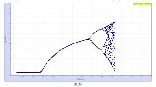
The behavior of the logistic equation depends on the value of the growth parameter, r. If the growth parameter is less than a critical value r<0.75..., then x approaches a stable fixed value. Above this value for r, the behavior of x begins to change. First the population begins to oscillate between two values. If r increases further, then x oscillates between four values, then eight values. This doubling ends when r > 0.8924864... after which almost any x value is possible.

Generalized logistic map

x_n+1 = 4rx_n(1-x_n) = 4 r ( x_n -x_n²)

The logistic series rule sets the next generation proportional to the existing one in its first term. This alone would lead to exponential growth for r > 1/4, and to exponential decline for r < 1/4). The second term introduces a diminution that depends on the square of the existing population (note that in the above formulation x_n < 1 , hence x_n² < x_n ).

The issue for a given growth rate r is:  will the population approach a stable equilibrium (limit) value of linear growth and quadratic extinction − assuming an unlimited number of generations under identical conditions. If so, how does the equilibrium value depend on the growth rate r ?

Growth exists when x_n+1 > x_n, hence r > 1/(4(1-x_n)). As 0 < x < 1 , for r < 0.25, all populations will iterate to zero, independent of the starting value. If for r > 0.25 an equilibrium value exists, a starting population greater than the limit should shrink to it, smaller ones should expand to it.

In the simulation r is increased in steps of 0.001 in the range 0 < r < 1 . The calculation for each step starts with a random value 0 < x₁< 1 . In a calculation loop 2000 members of the series are calculated. The first ones differ largely in dependence on the random initial value. Therefore the first 1000 iterations are suppressed in the chart. For each step in r 1000 points on the ordinate could represent the iterations 1000 to 2000.

In the range 0.25 < r < 0.75 the iterations are so close together that they appear as one point only, resulting in a "limit curve" in dependence on r.

Then the curve splits in two (bifurcation), which means that the iteration now has two accumulation points for a certain r. The bifurcation repeats itself, until no accumulation points are visible any longer.

Quite surprisingly between the "filled" bands there are some quasi "empty" bands with only a few accumulation points.

The determining term is the product 4r; factors different from 4 just scale the abscissa differently.

It is not decisive for the bifurcation that the limiting term is exactly (1-x_n). The crucial point is the nonlinearity of the conjunction x_n -x_n².

To demonstrate this, a generalized series rule is used in this simulation, using a term (1-x_n^k), with k > 0 :

x_n+1 = 4rx_n(1-x_n^k)

When opening the simulation k =  1; Start produces the common logistic map.

After Stop k can be changed in the range 0.1 < k < 2 by a slider. The abscissa scaling is adjusted automatically.

The left chart displays the total range, the right one that of bifurcation with higher resolution. One can differentiate the calculation steps and the bifurcation structure in more detail if the window is expanded to full screen size.

Author von LogisticMap.xlm : Francisco Esquembre and Wolfgang Christian.

Text and original idea from the Open Source Physics project manual

Date : July 2003

Generalized by Dieter Roess in August 08

This simulation is part of

“Learning and Teaching Mathematics using Simulations

– Plus 2000 Examples from Physics”

ISBN 978-3-11-025005-3, Walter de Gruyter GmbH & Co. KG

 

Translations

Code	Language		Translator	Run

Credits

Dieter Roess - WEH- Foundation; Tan Wei Chiong; Lookang Wee; Wolfgang Christian; Francisco Esquembre

Overview:

This document provides a briefing on the Logistic Map JavaScript Simulation Applet, an interactive resource from Open Educational Resources / Open Source Physics @ Singapore. The applet is designed to visually demonstrate the behavior of the logistic map, a fundamental concept in the study of dynamical systems and chaos theory. This briefing will outline the core concepts of the logistic map, the features of the simulation, and its pedagogical applications.

Main Themes and Important Ideas/Facts:

• The Logistic Map as a Population Dynamics Model: The logistic map is introduced as a "simple model of population dynamics" first proposed by Robert May. It's represented by a one-dimensional difference equation:
• Equation: xn+1 = 4 r xn (1-xn)
• Here, xn represents the population in one generation (scaled between 0 and 1), and xn+1 represents the population in the succeeding generation. The parameter 'r' is the growth rate.
• Dependence on the Growth Parameter (r): The behavior of the logistic equation is highly dependent on the value of the growth parameter 'r' (in the simulation, this 'r' ranges from 0 to 1, effectively a scaled version where the original 'r' is 4 times this value).
• Stable Fixed Point: For lower values of 'r' (specifically, r < 0.75 in the original 'r' scaling, which corresponds to a different range in the simulation's 0-1 'r'), the population 'x' approaches a "stable fixed value."
• Oscillations and Bifurcation: As 'r' increases beyond this critical value, the behavior changes. The population starts to oscillate between two values. Further increases in 'r' lead to oscillations between four, then eight values. This "doubling" or bifurcation continues.
• Onset of Chaos: The period-doubling cascade ends when r > 0.8924864.. (in the original 'r' scaling). Beyond this point, the system exhibits chaotic behavior, where "almost any x value is possible," meaning unpredictable fluctuations.
• Generalized Logistic Map: The simulation also includes a generalized form of the logistic map:
• Equation: xn+1 = 4rxn(1-xnk)
• This generalization introduces a term (1-xnk) where 'k' can be varied (k > 0). The simulation allows users to adjust 'k' using a slider after stopping the initial run (where k = 1 for the standard logistic map).
• The document emphasizes that the "crucial point is the nonlinearity of the conjunction xn -xn2 *" (in the standard form) and that the exact form of the limiting term (1-xn) is not as critical as its nonlinearity for the emergence of bifurcation and chaos.
• Simulation Features:The simulation allows users to vary 'r' in steps of 0.001 within the range 0 to 1.
• For each 'r' value, it calculates 2000 iterations of the logistic map, starting with a random initial population (0 < x1 < 1).
• To focus on the long-term behavior, the first 1000 iterations are suppressed in the visual chart, displaying the subsequent 1000 points.
• The simulation visually represents the iterations against the 'r' parameter. In the stable range (0.25 < r < 0.75 in the simulation's 'r'), the iterations appear as a single "limit curve."
• The simulation visually demonstrates the bifurcations as the 'r' value increases, where the "limit curve" splits into two, then four, and so on.
• The simulation highlights the surprising presence of "quasi 'empty' bands with only a few accumulation points" within the chaotic regions.
• The generalized map allows exploration of how changing the exponent 'k' in (1-xnk) affects the dynamics and bifurcation structure.
• Two charts are provided: one showing the total range and another with higher resolution for the bifurcation region.
• Pedagogical Applications:The resource is designed for "Learning and Teaching Mathematics using Simulations."
• It provides a visual and interactive way to understand concepts like sequences, series, stability, oscillations, bifurcation, and chaos.
• The "For Teachers" section explicitly states that the "Logistic Map is commonly used to show how chaotic systems can arise from seemingly simple models."
• It can be used to illustrate the effects of reproduction (proportional growth at small populations) and starvation (decrease proportional to carrying capacity).
• Authorship and Credits:The original idea and text are attributed to the Open Source Physics project manual by Francisco Esquembre and Wolfgang Christian (July 2003).
• The generalization was done by Dieter Roess in August 2008.
• The JavaScript version was created by Wei Chiong and Loo Kang (2018).
• The project acknowledges contributions from various individuals and the WEH- Foundation.
• Technical Aspects:The applet is implemented in HTML5 and JavaScript, making it embeddable in webpages using an <iframe> tag.
• The use of the term 4r in the equation within the simulation (where 'r' ranges 0-1) is clarified for teachers, explaining it's a scaling of the original growth parameter.

Key Quotes:

• "The logistic equation was first proposed by Robert May as a simple model of population dynamics."
• "If the growth parameter is less than a critical value r<0.75 ..., then x approaches a stable fixed value. Above this value for r, the behavior of x begins to change. First the population begins to oscillate between two values. If r increases further, then x oscillates between four values, then eight values. This doubling ends when r > 0.8924864.. after which almost any x value is possible."
• "It is not decisive for the bifurcation that the limiting term is exactly (1-xn ) . The crucial point is the nonlinearity of the conjunction xn -xn2 ."
• "When r is approximately 0.89 to 1, the population size starts to exhibit chaotic behaviour, fluctuating wildly between many values. In fact, the Logistic Map is commonly used to show how chaotic systems can arise from seemingly simple models."

Conclusion:

The Logistic Map JavaScript Simulation Applet is a valuable educational tool for demonstrating the complex dynamics that can emerge from a simple nonlinear equation. By allowing users to interactively explore the impact of the growth parameter 'r' and the generalization factor 'k', it provides an intuitive understanding of concepts like stability, bifurcation, and the onset of chaos. Its accessibility as an HTML5 applet makes it easily integrable into online learning environments.

 

Logistic Map Study Guide

Key Concepts

• Logistic Equation: The fundamental equation xn+1 = 4rxn(1-xn) used to model population dynamics.
• Population Dynamics: The study of how populations of organisms change in size and composition over time.
• Difference Equation: A mathematical equation that relates the values of a sequence at different time steps.
• Growth Parameter (r): A value that influences the behavior of the logistic equation and determines the rate of population growth. In this simulation, r ranges from 0 to 1 (representing 4r in the standard form).
• Stable Fixed Value: A state where the population size eventually settles to a single, constant value over many generations. This occurs at lower values of r (< 0.75).
• Oscillation: A pattern where the population size repeatedly fluctuates between a set of values. The number of values in the cycle increases (period-doubling) as r increases.
• Bifurcation: The splitting of the "limit curve" in the simulation, indicating a change from a stable fixed point to oscillations between multiple values.
• Limit Curve: The visual representation in the simulation where iterations appear as a single point, indicating a stable equilibrium for a given r.
• Chaotic Behavior: Irregular and unpredictable fluctuations in population size that occur at higher values of r (> approximately 0.8924864). Almost any population value becomes possible.
• Nonlinearity: The presence of terms like xn^2 in the logistic equation, which is crucial for the complex behaviors observed, including bifurcations and chaos.
• Generalized Logistic Map: An extension of the basic logistic equation, xn+1 = 4rxn(1-xn^k), where k is a parameter that can be adjusted to demonstrate the importance of nonlinearity.
• Iteration: A single step in the calculation of the logistic map, representing the transition from one generation to the next.
• Equilibrium Value: A stable population size that the system approaches over many iterations.
• Domain of x: The range of possible population values, which is [0, 1] in the scaled logistic equation used here.
• Carrying Capacity: The maximum population size that an environment can sustain indefinitely. The (1-xn) term in the logistic equation models limitations imposed by carrying capacity.

Short Answer Quiz

1. What is the basic form of the logistic equation presented in the source, and what do the terms xn+1 and xn represent? The logistic equation is xn+1 = 4rxn(1-xn). Here, xn represents the population in the current generation, and xn+1 represents the population in the succeeding generation.
2. According to the text, what happens to the population when the growth parameter r is below a critical value (approximately < 0.75)? When the growth parameter r is below a critical value (around 0.75), the population x approaches a stable fixed value over successive generations. This means the population size eventually settles to a constant level.
3. Describe the behavior of the population as the growth parameter r increases beyond the critical value, according to the source. As r increases beyond the critical value, the population's behavior changes from reaching a stable fixed point to oscillating between two values. With further increases in r, the oscillations double to four, then eight values, eventually leading to chaotic behavior.
4. What is meant by "bifurcation" in the context of the logistic map simulation? Bifurcation refers to the splitting of the "limit curve" observed in the simulation as the growth parameter r increases. This splitting indicates that the population no longer settles on a single value but oscillates between two distinct accumulation points.
5. Explain the role of the term (1-xn) in the logistic equation in terms of population dynamics. The term (1-xn) introduces a diminution or constraint on population growth, which is proportional to the square of the existing population. This factor models the effects of carrying capacity and resource limitations, preventing unlimited exponential growth.
6. What is the significance of the nonlinearity in the logistic equation (xn - xn^2) for the complex behaviors observed? The nonlinearity, specifically the presence of the xn^2 term, is crucial for generating the complex dynamics such as oscillations and chaos. Without this nonlinearity, the model would only exhibit exponential growth or decline.
7. What happens to the population when the growth rate r is less than 0.25, according to the text? When the growth rate r is less than 0.25, all populations will iterate to zero, regardless of the initial starting population value. This indicates a consistent population decline to extinction.
8. What range of r in the simulation is associated with chaotic behavior in the population? Chaotic behavior in the population is generally observed in the simulation when the growth parameter r is approximately between 0.89 and 1. In this range, the population fluctuates wildly and unpredictably.
9. What does the generalized logistic map (xn+1 = 4rxn(1-xn^k)) allow users to investigate in the simulation? The generalized logistic map allows users to investigate the effect of changing the exponent k in the (1-xn^k) term. This demonstrates that the crucial factor for bifurcation and chaos is the nonlinearity of the term, rather than it being strictly (1-xn).
10. How does the simulation handle the initial iterations, and why? The simulation suppresses the first 1000 iterations in the chart because these initial values can differ significantly depending on the random starting population. Focusing on iterations 1000 to 2000 allows for observation of the long-term behavior and patterns that emerge.

Essay Format Questions

1. Discuss how the logistic map, despite its simplicity as a one-dimensional difference equation, can model complex population dynamics, including stable equilibria, oscillations, and chaos. Explain the role of the growth parameter r in these different behaviors.
2. Explain the concept of bifurcation in the context of the logistic map. Describe the sequence of bifurcations that occur as the growth parameter r is increased, and discuss the transition to chaotic behavior.
3. The source highlights the importance of nonlinearity (xn - xn^2) in the logistic map. Elaborate on why this nonlinearity is essential for the emergence of complex dynamics like period-doubling and chaos, and how the generalized logistic map (with the term (1-xn^k)) demonstrates this point.
4. Consider the applications of the logistic map beyond simple population dynamics. Based on the behaviors it exhibits, in what other scientific or mathematical fields might similar models or principles be relevant? Provide examples and explain your reasoning.
5. Describe the design and purpose of the JavaScript simulation applet for the logistic map. How does the interactive nature of the simulation, including the ability to adjust the growth parameter r and the exponent k, contribute to understanding the behavior of the logistic equation?

Glossary of Key Terms

• Logistic Equation: A mathematical formula, xn+1 = 4rxn(1-xn), that models population growth with resource limitations.
• Population Dynamics: The branch of biology that studies the size and age composition of populations as dynamic systems, and the biological and environmental processes driving them (such as birth and death rates, and immigration and emigration).
• Difference Equation: A recursive formula where the next term in a sequence is defined based on previous terms.
• Growth Parameter (r): A constant value in the logistic equation that influences the rate at which a population grows or declines.
• Stable Fixed Value (Equilibrium): A state in a dynamical system where the variables do not change over time; in the logistic map, a population size that remains constant after many iterations.
• Oscillation (Periodic Behavior): A repetitive fluctuation in the values of a system over time, cycling through a set of states.
• Bifurcation: A qualitative change in the behavior of a dynamical system as a parameter is varied, such as the splitting of a stable state into multiple oscillating states.
• Limit Curve: In the context of the logistic map simulation's bifurcation diagram, a visual representation of the long-term values (attractors) of the population for different values of the growth parameter.
• Chaotic Behavior (Chaos): A state in a dynamical system characterized by extreme sensitivity to initial conditions, leading to seemingly random and unpredictable behavior despite being governed by deterministic equations.
• Nonlinearity: A property of a system where the output is not directly proportional to the input, often involving terms of higher degree (e.g., squared or cubed variables).
• Generalized Logistic Map: An extension of the standard logistic equation that introduces an additional parameter k to modify the nonlinearity.
• Iteration: A single execution of the logistic equation, calculating the population for the next generation based on the current generation's population.
• Domain: The set of all possible input values for a function or model; in the logistic map, the possible values for the population x (0 to 1).
• Carrying Capacity: The maximum population size that an environment can sustainably support given the available resources.

For Teachers

The Logistic Map is used to model population growth using the following equation: x(n+1) = rx(n)(1 - x(n))

Where x represents the ratio of the existing population to the maximum possible population, n represents the number of iterations, and r is a parameter ranging between 0 and 4 that changes the behaviour of the population growth.

In this simulation, we denote the parameter r by 4r, where r now ranges between 0 and 1. From here on, when we refer to r, we mean the r in the simulation that ranges between 0 and 1.

This model simulates the effects of reproduction, where the population size increases at a rate proportional to the current population when the population is small, and starvation, where the population size decreases at a rate proportional to the carrying capacity of the environment.

It is not decisive for the bifurcation that the limiting term is exactly (1-x(n)). The crucial point is the non-linearity of the conjunction x(n) -x(n)^2.

To demonstrate this, a generalized series rule is used in this simulation, using a term (1-x(n)^k), with k > 0 :
x(n+1) = 4rx(n)(1-x(n)^k)

When r is approximately 0.89 to 1, the population size starts to exhibit chaotic behaviour, fluctuating wildly between many values. In fact, the Logistic Map is commonly used to show how chaotic systems can arise from seemingly simple models.

Author : Francisco Esquembre and Wolfgang Christian, JavaScript version Wei Chiong and Loo Kang
Text and original idea from the Open Source Physics project manual
Date : July 2003 and JavaScript 2018

Video

[text]

 Version:

1. http://phy01.phy.ntnu.edu.tw/ntnujava/index.php?topic=1817.0
2. https://weelookang.blogspot.com/2018/05/logistic-map-javascript-simulation.html 

Other Resources

[text]

Frequently Asked Questions about the Logistic Map Simulation

• What is the logistic map and what does it model? The logistic map is a mathematical equation, specifically a one-dimensional difference equation, introduced by Robert May as a simple model of population dynamics. It describes how the population in one generation ($x_n$) transforms into the population of the next generation ($x_{n+1}$) using the formula $x_{n+1} = 4rx_n(1-x_n)$. Here, $x_n$ represents the ratio of the existing population to the maximum possible population (scaled between 0 and 1), and $r$ is the growth parameter that influences the population's behavior.
• How does the growth parameter 'r' affect the behavior of the logistic map? The behavior of the population in the logistic map is highly dependent on the value of the growth parameter $r$ (which ranges from 0 to 1 in this simulation, corresponding to a factor of $4r$ in the original formulation where $r$ ranged from 0 to 4).
• For $r < 0.25$, the population will always decline to zero, regardless of the initial population.
• For $0.25 < r < 0.75$, the population will eventually approach a stable, fixed equilibrium value (a "limit curve").
• As $r$ increases beyond approximately 0.75, the population starts to oscillate between two values. Further increases in $r$ lead to oscillations between four, then eight values, and so on, in a process called bifurcation.
• This period-doubling cascade ends around $r \approx 0.8924864...$.
• For $r$ values above this, the system exhibits chaotic behavior, where the population fluctuates wildly between many possible values, and even slight changes in the initial population can lead to drastically different long-term outcomes.
• What is the significance of the term (1 - xn) in the logistic equation? The first term in the equation, $4rx_n$, represents population growth proportional to the current population, which alone would lead to exponential growth (for $r > 1/4$) or decline (for $r < 1/4$). The second term, $(1 - x_n)$, introduces a density-dependent limitation on growth. As the population ($x_n$) approaches the maximum carrying capacity (1), the term $(1 - x_n)$ approaches zero, thus slowing down and eventually reversing population growth. This can be interpreted as representing factors like limited resources or increased competition as the population size increases.
• What is bifurcation in the context of the logistic map? Bifurcation in the logistic map refers to the splitting of the long-term behavior of the population as the growth parameter $r$ is increased. Instead of settling on a single stable value, the population begins to oscillate between two distinct values at a certain critical $r$. As $r$ is further increased, this oscillation period doubles (to four values, then eight, and so on). These points where the stable behavior splits into multiple stable states are called bifurcation points. This sequence of period-doubling bifurcations is a characteristic feature of the transition to chaos in many dynamical systems.
• What is meant by "chaotic behavior" in the logistic map? In the context of the logistic map, chaotic behavior occurs when the growth parameter $r$ is sufficiently high (approximately above 0.89 in this simulation's scaling). In this regime, the population size no longer settles into a predictable cycle or a stable equilibrium. Instead, it fluctuates seemingly randomly between many different values. A key characteristic of chaotic systems, including the logistic map in this range, is their sensitivity to initial conditions. Even infinitesimally small differences in the starting population can lead to vastly different population trajectories over time, making long-term prediction impossible.
• Is the specific form (1 - xn) crucial for observing bifurcation and chaos in this model? No, the exact form of the limiting term $(1 - x_n)$ is not the crucial factor for observing bifurcation and chaos. The essential aspect is the nonlinearity introduced by the term $x_n - x_n^2$. The simulation allows exploring a generalized form $(1 - x_n^k)$, where $k > 0$. Changing the value of $k$ modifies the specific dynamics and scaling but the fundamental phenomenon of bifurcation and the emergence of chaos due to this nonlinearity remains.
• How is the simulation designed to illustrate the behavior of the logistic map? The JavaScript simulation allows users to vary the growth parameter $r$ (in steps of 0.001 from 0 to 1). For each value of $r$, it starts with a random initial population ($0 < x_1 < 1$) and iterates the logistic equation 2000 times. To focus on the long-term behavior, the first 1000 iterations (which can be heavily influenced by the random starting value) are suppressed in the chart. The subsequent 1000 iterations (representing the behavior after the system has settled) are plotted. For certain ranges of $r$, these iterations cluster closely, forming a "limit curve." Bifurcations are visualized as this curve splitting into multiple branches, indicating oscillations between different population values. The chaotic regime is seen where the plotted points fill vertical bands, showing the wide range of possible population values.
• What are some of the key concepts that can be learned using this logistic map simulation? This simulation provides a visual and interactive way to understand several important concepts in mathematics and science, including:
• Nonlinear Dynamics: How simple nonlinear equations can lead to complex and unpredictable behavior.
• Equilibrium and Stability: The concept of stable fixed points and how they depend on parameters.
• Bifurcation: The qualitative changes in a system's behavior as a parameter is varied.
• Period Doubling: A common route to chaos where oscillations double in period.
• Chaos Theory: The characteristics of chaotic systems, such as sensitivity to initial conditions and seemingly random behavior despite deterministic rules.
• Mathematical Modeling of Population Dynamics: How mathematical equations can be used to model real-world phenomena, even if those models are simplifications.