About

Description of the simulation window

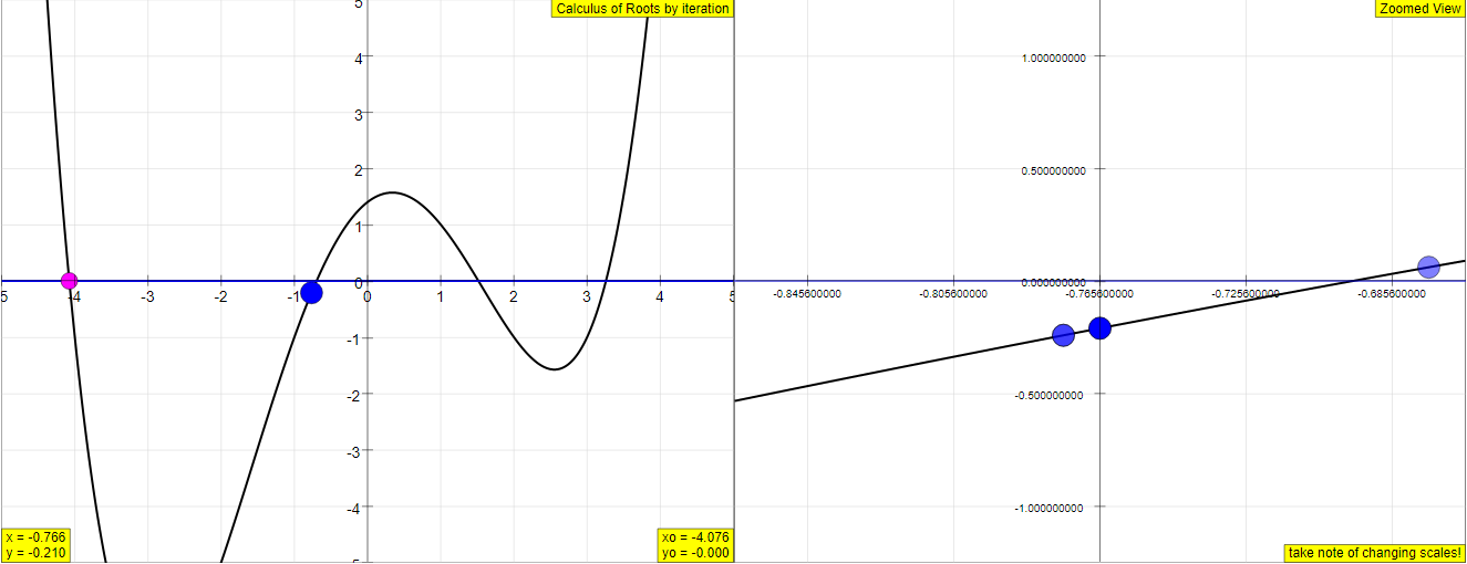
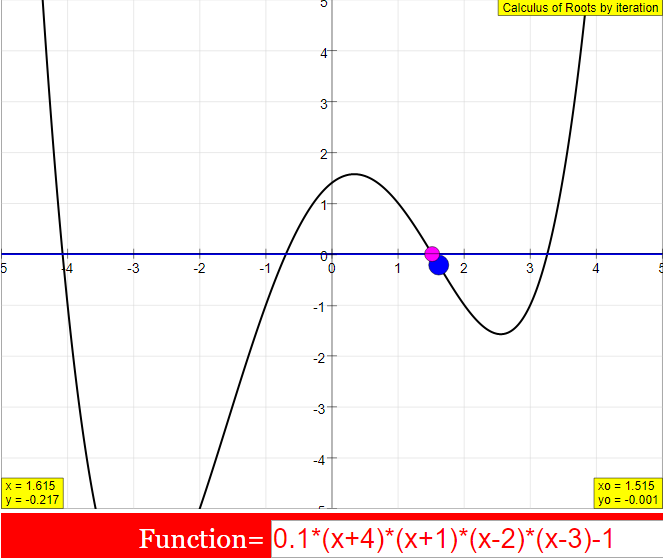
The simulation has two windows with an x, y coordinate system. As default the left one shows a power function (parabola) of fourth grade. Its roots are to be calculated (the x values for which y is zero). Its formula is visible in a text field:

y =  0.1(x+4)(x+1)(x-2)(x-3)-0.1

= 0.1(x⁴ - 3x² + 10x + 23)

The first formulation indicates that there are 4 roots which are near to the integers -4, -1, 2 and 3. Substituting the constant element (-0.1) by 0, these integers would be exact solutions. The roots of the predefined function are irrational numbers.

The range of the x coordinate goes from -x_max to +x_max. The default value of x_max is 5; it can be changed in the number field. The range of the y coordinate goes from -12 to +12. Changing to another y scaling is achieved by using appropriate factors (default 0,1) in the editable formula.

The magenta colored point is the starting point of the calculation (default x₀= - 4.5). It can be drawn with the mouse along the function curve to another abscissa. While the blue iteration points wanders along the curve in the positive x direction, the starting point stays fixed till a root has been calculated with the required accuracy delta. Then it will jump to this root.

The required deviation from exactly zero delta = y -0 can be defined in the white number field (default 0.00001). The current deviation during the calculation process is shown in the gray y field below. Two gray number fields retain the values xo and y0 of the initial point and hence also of the last root found.

The current iteration point is shown in blue. Once a root has been calculated with the required precision, it jumps to the first point of the next iteration.

At high accuracy, the movement of the iteration point will no longer be recognizable after a few iteration steps. For this reason the right window shows a zoomed section of the curve with self adjusting scales. Up o 4 consecutive points of the iteration are retained, the current one blue, three trailing ones in red (after a flyback blue and red coincide for one point).

In the zoom window one can follow the flybacks of the iteration process and the reduction of the x step by a factor of 10 at such an event up to the highest resolution. During this process the curve will appear more and more like a straight line.

The Start/ Stop button controls the iteration process. Restart leads back to the default situation. The number of iteration steps per second is defined by the slider speed between 1 and 25 (default 2). Default stops the iteration when a root has been found; to get the next one shift the initial point with the mouse and Start again. Refusing the Option One root only calculates all roots in consecutve order.

The speed of the Simulation is determined by the stepwise time control of visualization. It has no relation to the very short time interval which the computer would need to calculate a new root without these interruptions

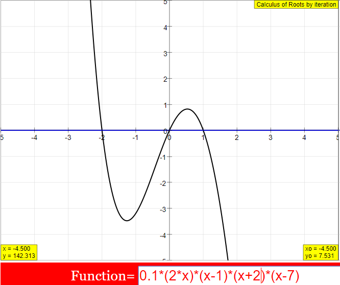
The text field of the formula is editable. You can input any formula to determine its roots. Take care to adjust x_max and the ordinate scale to the specifics of the function.

Iteration algorithm

The equation f(x) = g(x)

can be formulated as f(x) - g(x) = 0

Hence the general task to determine conditions of equality of 2 functions for a value x is reduced to finding the roots of one equation, where its value is zero. If g(x) is a number q, the task is to find a value x for which f(x) has the value q.

Logically the task presents the inversion of the simple task to calculate the value of f(x) for a given x. Yet an analytic solution is possible only for very simple functions, as a linear or a second order parabola. With trigonometric functions or logarithms, in classical technique, we use tables of corresponding numbers, without normally asking how they originated.

Numerically the roots of any function can be calculated by iteration up to every wanted, finite degree of accuracy. Instead of looking for an inverting calculus, we simply calculate "forward". We take an initial arbitrary value of x and calculate y = f(x). In general y will not be zero, and hence x will not be a root. Now we vary x systematically (iterate x) until y becomes smaller than a desired accuracy delta.

For easy understanding and demonstration this simulation uses a very simple iteration algorithm in form of a calculating loop. In each step of the loop the following commands are performed (you will find the code at the Evolution page of the EJS model);

d x = 0.1/n; defines the step width in dependence on a step variable n

x = x + dx; goes one step further

the corresponding y- value is calculated with the given formula for f(x) (Fixed Relations page)

if (y>0) ( it is assumed that initially y<0, with changing sign (y>0) a root has been crossed) {

x = x - 2*dx; jump back to last point

n=10*n; reduce step by factor 10

}

if (Math.abs(y)<2*delta) when y is sufficiently small {

_pause(); -stop calculation

}

While this algorithm is very simple and easy to understand, it needs many steps. One can speed it up considerably using variable step widths, that adjust themselves to the steepness of the curve or even to its curvature. In the zoom window one recognizes that the function can quickly be approximated well by a linear. The root of a linear determined by 2 consecutive points of the iteration or even of a parabola determined by 3 of them, will be very close to the root of the curve itself after just one more step of iteration. The linear approximation is used in the so called Newton algorithm.

With the availability of fast PCs the time needed for iteration algorithms is so minute that one can use them universally. Standard programs like Excel or Mathematica offer ready solutions.

Our simple algorithm is easily extended to calculate all roots in a given interval in one run. An additional if- else- logic condition is sufficient to adjust the flyback command to the 2 cases of the initial y value being positive or negative.

if (y0<0) {

dx = 0.1/n;

x = x + dx;

if (y > 0) {

x = x - 2*dx;

n = 10*n;

}}

else {

dx = 0.1/n;

x = x + dx;

if (y < 0) {

x = x - 2*dx;

n =10*n;

}}

As the formula field is editable, one can determine roots for any arbitrary function.

E1: Start the default situation. Watch the flybacks with changing step width in the zoom window, and the changes in the number fields.

E2: After Reset increase speed to 10. In the zoom window the consecution of the iteration point, the formation of the trailing followers and the jump back after crossing a root will be better recognizable.

E4: Change speed to 1. Stop iteration after a flyback. Using the Start/Stop button you can now follow single steps. In the zoom window you can follow the jumps in scaling of both abcissa and ordinate.

E5: Change speed while the iteration runs.

E6: Change the residual value delta over a wide range and control if it is really achieved.

E7: Draw the initial point and calculate the 4 roots separately this way.

E8: Delete the constant element in the formula window. Now the roots should be integers. Control the achieved accuracy!

E9: Change the formula in the formula field to 10*sin(x) (factor 10 for adjustment to the y scale). Calculate the first root. Repeat the calculation for different values of delta. Compare the results to π = 3.14159 26535 89793...

E10: Calculate roots for functions of your own.

 

Translations

Code	Language		Translator	Run

Credits

Dieter Roess - WEH-Foundation; Fremont Teng; Loo Kang Wee

Overview:

This document provides a review of the "Calculus of Roots by Iteration JavaScript Simulation Applet HTML5" resource. This interactive tool aims to help users learn and visualize the numerical method of finding the roots (the x values for which y equals zero) of a given function through iterative calculations. The applet features a customizable function, adjustable parameters for the iteration process, and graphical representations to illustrate the steps involved.

Main Themes and Important Ideas/Facts:

1. Numerical Root Finding by Iteration: The core concept demonstrated by the applet is the numerical method of finding roots. Unlike analytical solutions which are only possible for simple functions, numerical methods use iterative processes to approximate the roots to a desired degree of accuracy. The document states, "Numerically the roots of any function can be calculated by iteration up to every wanted, finite degree of accuracy."
2. Simulation Window and Function Representation: The simulation features two linked graphical windows. The left window displays the function, with a default being a fourth-grade polynomial: "y = 0.1(x+4)(x+1)(x-2)(x-3)-0.1". The user can observe the curve and the iteration points in this window. The formula is editable, allowing users to input their own functions. The document highlights, "The text field of the formula is editable. You can input any formula to determine its roots."
3. Iterative Algorithm: The applet employs a straightforward iterative algorithm. Starting with an initial guess (x0), the algorithm iteratively steps along the x-axis, calculating the corresponding y value. The key steps of the implemented algorithm are:

• Defining a step width: "d x = 0.1/n"
• Incrementing x: "x = x + dx"
• Calculating the new y value based on the function.
• Checking for root crossing: "if (y>0) (it is assumed that initially y<0, with changing sign (y>0) a root has been crossed) { x = x - 2*dx; n=10n*; }" - This indicates a "flyback" where the step size is reduced when a root is likely crossed.
• Checking for desired accuracy: "if (Math.abs(y)<2delta*) when y is sufficiently small { _pause(); -stop calculation }" - The iteration stops when the absolute value of y is less than twice the defined accuracy delta.

1. Zoom Window for Detail: The right window provides a zoomed-in view of the curve around the iteration points. This is crucial for visualizing the behavior of the algorithm at high accuracy where the movement in the main window becomes imperceptible. The document explains, "For this reason the right window shows a zoomed section of the curve with self adjusting scales. Up o 4 consecutive points of the iteration are retained, the current one blue, three trailing ones in red..."
2. User Control and Parameters: The simulation offers several interactive controls:

• Editable Formula: Users can input any function.
• xmax: Adjustable range for the x-axis.
• Initial Point (magenta): Can be dragged along the curve to start the iteration from different x values. The document notes, "The magenta colored point is the starting point of the calculation (default x0 = - 4.5) . It can be drawn with the mouse along the function curve to another abscissa."
• Delta: Defines the required accuracy (deviation from zero) for a root. "delta = y -0 can be defined in the white number field (default 0.00001 )."
• Speed Slider: Controls the number of iteration steps per second.
• Start/Stop Button: Initiates and halts the iteration process.
• Restart Button: Resets the simulation to its default state.
• One root only Checkbox: When unchecked, the simulation will attempt to find all roots consecutively.

1. Comparison to More Advanced Algorithms: While the simulation uses a simple iteration method for clarity, the document acknowledges that more efficient algorithms exist. "While this algorithm is very simple and easy to understand, it needs many steps. One can speed it up considerably using variable step widths, that adjust themselves to the steepness of the curve or even to its curvature. [...] The linear approximation is used in the so called Newton algorithm."
2. Practical Applications and Tools: The text mentions that iteration algorithms are now widely applicable due to the speed of modern computers and are integrated into standard software like "Standard programs like Excel or Mathematica offer ready solutions."
3. Experiments for Learning: The resource includes a section on "Experiments" suggesting various ways users can interact with the simulation to understand the concepts better. These experiments involve changing parameters like speed, delta, the initial point, and the function itself. For instance, "E9: Change the formula in the formula field to 10sin(x)* ... Calculate the first root. Repeat the calculation for different values of delta. Compare the results to π = 3.14159 26535 89793..."
4. For Teachers: A section "For Teachers" provides brief instructions on using the interface elements like the speed slider, delta field, function box, and pause at root checkbox, indicating its potential as a teaching tool.

Key Quotes:

• "Its roots are to be calculated (the x values for which y is zero)."
• "The text field of the formula is editable. You can input any formula to determine its roots."
• "Numerically the roots of any function can be calculated by iteration up to every wanted, finite degree of accuracy."
• "For easy understanding and demonstration this simulation uses a very simple iteration algorithm in form of a calculating loop."
• "While this algorithm is very simple and easy to understand, it needs many steps. One can speed it up considerably using variable step widths..."
• "Standard programs like Excel or Mathematica offer ready solutions."

Conclusion:

The "Calculus of Roots by Iteration JavaScript Simulation Applet HTML5" provides a valuable interactive platform for understanding the fundamental principles of numerical root-finding using iterative methods. Its clear visual representation, user-friendly controls, and the ability to customize the function make it an effective tool for both learning and teaching mathematics. While the algorithm used is simple for demonstration purposes, the resource acknowledges the existence of more advanced techniques. The inclusion of suggested experiments further enhances its educational value.

 

Calculus of Roots by Iteration Study Guide

Key Concepts

• Roots of a function: The values of x for which the function y = f(x) equals zero. These are the points where the graph of the function intersects the x-axis.
• Iteration: A process of repeating a set of instructions or calculations to obtain a desired result. In this context, it involves systematically changing the value of x to get closer to a root of the function.
• Numerical method: A technique used to find approximate solutions to mathematical problems that are difficult or impossible to solve analytically. The iteration algorithm described is a numerical method for finding roots.
• Step width (dx): The size of the increment or decrement applied to the value of x in each iteration step. The simulation uses a step width that changes based on the proximity to a root.
• Flyback: The action of the iteration point moving back after crossing a root, indicated by a change in the sign of the y value. This triggers a reduction in the step width.
• Accuracy (delta): The maximum allowed deviation from zero for the y value. The iteration process stops when the absolute value of y is less than 2delta, indicating a root has been found within the desired precision.
• Iteration algorithm: The specific set of instructions or rules followed in each step of the iteration process to find a root. The simulation uses a simple algorithm involving stepping, checking the sign of y, and adjusting the step width.
• Zoom window: A separate display in the simulation that shows a magnified view of the function curve around the current iteration point, allowing for a closer observation of the iteration process and flybacks.
• Initial point (x0, y0): The starting value of x chosen for the iteration process. The simulation allows the user to set this point by clicking on the function curve.

Quiz

1. What is a root of a function, according to the provided text? Describe how roots are visually represented on a graph.
2. Explain the concept of iteration as it is applied in the context of finding the roots of a function using this simulation.
3. Describe the simple iteration algorithm used in the simulation. What triggers the "flyback" of the iteration point, and what happens to the step width at this point?
4. What is the significance of the "delta" value in the simulation? How does this value relate to the accuracy of the calculated root?
5. Explain the purpose of the zoom window in the simulation. What information can be observed in this window that might not be as clear in the main window?
6. How can a user change the function for which the roots are to be calculated in the simulation? What considerations should be taken when changing the formula?
7. Describe how the "Start/Stop," "Restart," and "Default" buttons control the simulation. What is the difference between the "Default" behavior and refusing the "One root only" option?
8. Why does the right window (zoom window) show the curve appearing more and more like a straight line during the iteration process at high accuracy?
9. According to the text, what are some limitations of finding roots analytically, and how does numerical iteration provide a more universal approach?
10. Briefly describe one of the suggested experiments (E1-E10) and what a user might learn by performing it.

Quiz Answer Key

1. A root of a function is an x value for which the function's y value is zero. Visually, roots are the points where the graph of the function intersects or touches the x-axis.
2. Iteration in this context is a step-by-step numerical process of finding a root. Starting with an initial guess for x, the simulation repeatedly adjusts the x value and calculates the corresponding y value, aiming to make y as close to zero as possible.
3. The algorithm starts with a step width dx and incrementally changes x. If the y value changes sign (assumed from negative to positive), indicating a root has been crossed, the iteration point "flies back" by 2dx*, and the step width is reduced by a factor of 10.
4. The "delta" value represents the required deviation from exactly zero for the y value. The simulation stops the iteration when the absolute value of y is less than 2delta*, meaning the calculated x value is considered a root within the specified tolerance.
5. The zoom window provides a magnified view of the function curve around the current iteration point. This allows users to clearly see the individual iteration steps, the "flybacks," and the reduction in step width, which might be indistinguishable in the main window at high accuracy.
6. A user can change the function by editing the text in the "formula" field. When changing the formula, it's important to adjust the xmax value and the ordinate scale (by modifying factors in the formula) to appropriately display the new function and its potential roots.
7. The "Start/Stop" button initiates and pauses the iteration process. "Restart" resets the simulation to its default settings. "Default" stops the iteration once a single root is found, whereas refusing "One root only" allows the simulation to calculate all roots consecutively within the defined interval.
8. At high accuracy and in a very small interval around a root, most smooth functions can be well-approximated by a straight line (their tangent line). This is because the curvature becomes less significant at a very local scale.
9. Analytic solutions for roots are only possible for very simple functions like linear or second-order parabolas. For more complex functions, numerical iteration offers a general method to calculate roots to a desired degree of accuracy by repeatedly evaluating the function.
10. Experiment E9 suggests changing the formula to 10sin(x)* and calculating the first root, then comparing the result to π. By doing this, a user can observe how the iterative algorithm approximates a known root of the sine function and how the delta value affects the precision of the approximation.

Essay Format Questions

1. Discuss the advantages and limitations of using an iterative numerical method, such as the one described, for finding the roots of a function compared to analytical methods. Consider the types of functions for which each approach is most suitable.
2. Explain the role of the "flyback" mechanism and the reduction of step width in the simulation's algorithm. How do these features contribute to the accuracy and efficiency of finding roots?
3. Describe how the user interface of the JavaScript simulation applet facilitates the understanding of the root-finding iteration process. Refer to specific elements like the two windows, the color-coding, and the control buttons in your explanation.
4. The text mentions that more sophisticated iteration algorithms, like Newton's method, can significantly speed up the root-finding process. Based on the description of the simple algorithm used in the simulation, hypothesize how a method like Newton's, which uses linear approximation, might achieve faster convergence to a root.
5. Consider the educational value of using this interactive simulation for learning about the calculus of roots. How might experimenting with different functions, initial points, and accuracy settings enhance a student's understanding of this mathematical concept?

Glossary of Key Terms

• Abscissa: The x-coordinate of a point on a graph.
• Algorithm: A step-by-step procedure or set of rules to solve a problem.
• Analytic Solution: An exact solution to a mathematical problem expressed in terms of mathematical formulas and functions.
• Convergence: The tendency of an iterative process to approach a specific value (in this case, a root) as the number of iterations increases.
• Coordinate System: A system that uses one or more numbers, or coordinates, to uniquely determine the position of a point or other geometric element. The simulation uses a Cartesian (x, y) coordinate system.
• Deviation: The amount by which a value differs from a reference value (in this case, the difference between the function's value and zero).
• Function: A relation between a set of inputs and a set of permissible outputs with the property that each input is related to exactly one output.
• Irrational Number: A real number that cannot be expressed as a ratio of two integers.
• Ordinate: The y-coordinate of a point on a graph.
• Parabola: A symmetrical open plane curve formed by the intersection of a cone with a plane parallel to its side. The default function in the simulation is a quartic (fourth-degree) polynomial, the graph of which can have parabolic characteristics locally.
• Polynomial: An expression consisting of variables and coefficients, that involves only the operations of addition, subtraction, multiplication, and non-negative integer exponentiation of variables. The default function is a polynomial of the fourth degree.
• Precision: The degree of exactness with which a quantity is measured or calculated, often related to the number of significant figures. In the simulation, precision is related to the delta value.
• Simulation: A computer program that models the behavior of a real-world system or process.
• Step Variable (n): A variable used in the iteration algorithm to determine the current step width.
• Tangent Line: A straight line that touches a curve at a point such that its slope is equal to the slope of the curve at that point. Newton's method uses the tangent line to approximate the root.

Sample Learning Goals

[text]

For Teachers

Calculus of Roots by Iteration JavaScript Simulation Applet HTML5

Instructions

Speed Slider and Delta Field Box

Function Box

Pause at Root Check Box 

Toggling Full Screen

Play/Pause and Reset Buttons

Research

[text]

Video

[text]

 Version:

Other Resources

[text]

Frequently Asked Questions: Calculus of Roots by Iteration Simulation

• What is the purpose of this simulation? The simulation demonstrates a numerical method for finding the roots of a function, which are the values of x for which the function's output (y) is zero. It visualizes an iterative algorithm that systematically refines an initial guess until a root is found within a specified degree of accuracy.
• How does the iteration algorithm work in this simulation? The simulation employs a simple iterative loop. Starting from an initial x value, it calculates the corresponding y value using the given function. It then takes small steps in the positive x direction. If the sign of y changes (indicating a root has been crossed), it steps back, reduces the step size by a factor of 10, and continues the process until the absolute value of y is less than a defined accuracy threshold (delta).
• What can be manipulated in the simulation window? Users can interact with several elements:
• Formula Field: The mathematical function whose roots are to be found can be edited.
• xmax Field: The maximum value of the x-axis range can be adjusted.
• Initial Point: The starting x value for the iteration (magenta point) can be dragged along the function curve.
• Delta Field: The required accuracy (delta) for finding a root can be set.
• Speed Slider: The number of iteration steps per second can be controlled.
• Start/Stop Button: Initiates and pauses the iteration process.
• Restart Button: Resets the simulation to its default state.
• One root only Checkbox: Toggles whether the simulation stops after finding one root or continues to find subsequent roots.
• What do the different visual elements represent?
• Left Window: Displays the graph of the function over the defined x and y ranges. The magenta point is the initial guess, and the blue points represent the iteration steps.
• Right Window (Zoom): Shows a magnified view of the curve around the current iteration points, with self-adjusting scales to observe the refinement process. The current iteration point is blue, and the previous three are red (coinciding with blue after a flyback).
• Number Fields: Display the formula of the function, the current x and y values of the iteration, the initial x0 and y0 values (which retain the last found root), and the current deviation from zero (y).
• What is the significance of the "flybacks" and the changing step width? When the iteration crosses a root (indicated by a change in the sign of y), a "flyback" occurs where the iteration point jumps back. Simultaneously, the step width (dx) is reduced by a factor of 10. This process, visible in the zoom window, allows the algorithm to pinpoint the root with increasing precision.
• How does this iterative method relate to analytical methods for finding roots? Analytical methods for finding roots (like the quadratic formula) are only possible for certain simple types of functions (e.g., linear, quadratic). For more complex functions, finding roots analytically can be difficult or impossible. The numerical iterative method demonstrated here provides a way to approximate the roots of virtually any function to a desired degree of accuracy by repeatedly refining an initial estimate.
• What are some limitations and extensions of this simple iteration algorithm? The algorithm used in this simulation, while easy to understand, can be slow and require many steps to achieve high accuracy. More advanced numerical methods, such as the Newton-Raphson method, utilize information about the slope (and sometimes curvature) of the function to converge to a root much faster. The description mentions that the simple algorithm can be extended to find all roots within a given interval by adjusting the flyback logic based on the initial sign of y.
• What are some suggested experiments to explore the simulation? The provided text suggests several experiments, including: observing the default behavior, changing the speed of iteration, modifying the accuracy (delta), finding individual roots by adjusting the initial point, testing cases where roots should be integers, and exploring the roots of trigonometric functions like sin(x). Users are also encouraged to input their own functions to find their roots.