Breadcrumbs

About

Intro Page

The Wien (E x B) Filter

Developed by E. Behringer

This set of exercises guides the students to compute and analyze the behavior of a charged particle in a spatial region with mutually perpendicular electric and magnetic fields. It requires the student to determine the Cartesian components of hte forces acting on the particle and to obtain the corresponding equations of motion. The solutions to these equations are obtained through numerical integation, and the capstone exercise is the simulation of the (Wien) filter.

Subject Area	Electricity & Magnetism
Levels	First Year and Beyond the First Year
Available Implementation	Python
Learning Objectives	Students who complete this set of exercises will be able to: generate equations predicting the Cartesian components of force acting on the charged particle and generate the equations of motion for the particle (Exercise 1); calculate particle trajectories by solving the equations of motion (Exercise 2); produce two-dimensional and three-dimensional plots of the trajectories (Exercise 2); and simulate the operation of an (Wien) filter (Exercise 3) and determine the range of particle velocities transmitted by the filter, and how these are affected by the geometry of the filter (Exercise 4).
Time to Complete	120 min

Exercise 3

EXERCISE 3: THE (WIEN) FILTER, PART 1

Regions of mutually perpendicular electric and magnetic fields can be used to filter a collection of moving charged particles according to their velocity. If we assume that a particle of velocity enters the field region traveling exactly along the -axis, the particle will experience zero net force and therefore zero acceleration and zero deflection from the -axis. If a small, circular aperture of radius is placed on the -axis at , then this particle will be transmitted through the aperture.

(a) Use your program from Exercise 2 to determine the maximum value of for which an aperture of radius mm will transmit the Li ion (now assuming that ). What is the value of ?

(b) Repeat (a) for an aperture of radius mm. What is the value of ?

ExB_Filter_Exercise_3.py with Bug Fixes

# ExB_Filter_Exercise_3.py

# This file is used to numerically integrate

# the second order linear differential equations

# that describe the trajectory of a charged particle through

# an E x B velocity filter.

# Here, it is assumed that the axis of the filter

# is aligned with the z-axis, that the magnetic field

# is along the +x-direction, and that the electric field

# is along the -y-direction.

# The numerical integration is done using the built-in

# routine odeint

# The specific goal of this code is to identify the

# maximumm value of v_z that permits transmission of the

# particles through the velocity filter with

# a specified exit aperture.

# By:

# Ernest R. Behringer

# Department of Physics and Astronomy

# Eastern Michigan University

# Ypsilanti, MI 48197

# (734) 487-8799 (Office)

# ebehringe@emich.edu

# Last updated:

# 20160624 ERB

from pylab import figure,plot,xlim,xlabel,ylim,ylabel,grid,title,show,legend

from numpy import sqrt,array,arange,linspace,zeros,absolute

from scipy.integrate import odeint

# Initialize parameter values

q = 1.60e-19 # particle charge [C]

m = 7.0*1.67e-27 # particle mass [kg]

KE_eV = 100.0 # particle kinetic energy [eV]

Ex = 0.0 # Ex = electric field in the +x direction [N/C]

Ey = -105.0 # Ey = electric field in the +y direction [N/C]

Ez = 0.0 # Ez = electric field in the +z direction [N/C]

Bx = 0.002 # Bx = magnetic field in the +x direction [T]

By = 0.0 # By = magnetic field in the +x direction [T]

Bz = 0.0 # Bz = magnetic field in the +x direction [T]

R_mm = 1.0 # R = radius of the exit aperture [mm]

L = 0.25 # L = length of the crossed field region [mm]

u = [1.0,1.0,100.0]/sqrt(10002.0) # direction of the velocity vector

Ntraj = 1000 # number of trajectories

# Derived quantities

qoverm = q/m # charge to mass ratio [C/kg]

KE = KE_eV*1.602e-19 # particle kinetic energy [J]

R = 0.001*R_mm # radius of the exit aperture [m]

vmag = sqrt(2.0*KE/m) # particle velocity magnitude [m/s]

vzpass = -Ey/Bx # z-velocity for zero deflection [m/s]

# Set up the array of z-velocities to try

vz = vzpass + linspace(-0.25*vzpass,0.25*vzpass,Ntraj+1) # the set of initial z-velocities

particle_pass = zeros(Ntraj+1)

# Over what time interval do we integrate?

tmax = L/vzpass;

# Specify the time steps at which to report the numerical solution

t1 = 0.0 # initial time

t2 = tmax # final scaled time

N = 1000 # number of time steps

h = (t2-t1)/N # time step size

# The array of time values at which to store the solution

tpoints = arange(t1,t2,h)

# Here are the derivatives of position and velocity

def derivs(r,t):

# derivatives of position components

xp = r[1]

yp = r[3]

zp = r[5]

dx = xp

dy = yp

dz = zp

# derivatives of velocity components

ddx = qoverm*(Ex + yp*Bz - zp*By)

ddy = qoverm*(Ey + zp*Bx - xp*Bz)

ddz = qoverm*(Ez + xp*By - yp*Bx)

return array([dx,ddx,dy,ddy,dz,ddz],float)

# Specify initial conditions that don't change

x0 = 0.0 # initial x-coordinate of the charged particle [m]

dxdt0 = 0.0 # initial x-velocity of the charged particle [m/s]

y0 = 0.0 # initial y-coordinate of the charged particle [m]

dydt0 = 0.0 # initial y-velocity of the charged particle [m/s]

z0 = 0.0 # initial z-coordinate of the charged particle [m]

# Start the loop over the initial velocities

for i in range (0,Ntraj):

# Specify initial conditions

dzdt0 = vz[i] # initial z-velocity of the charged particle [m/s]

r0 = array([x0,dxdt0,y0,dydt0,z0,dzdt0],float)

# Calculate the numerical solution using odeint

r = odeint(derivs,r0,tpoints)

# Extract the 1D matrices of position values

position_x = r[:,0]

position_y = r[:,2]

# Check if the particle made it through the aperture

if absolute(position_x[N-1]) < R:

if absolute(position_y[N-1]) < sqrt(R*R - position_x[N-1]*position_x[N-1]):

particle_pass[i] = 1.0

else:

particle_pass[i] = 0.0

else:

particle_pass[i] = 0.0

# Look for the specific value of

for i in range (int(Ntraj/2),int(Ntraj)):#Frem:Added int

if absolute(particle_pass[i]-particle_pass[i-1]) > 0.5:

print("i = %d"%(i-1),"vz[i] = %.3e"%vz[i-1]," m/s.")#Frem:Added brackets

Deltav = vz[i-1] - vzpass

print("Delta v = %.3e"%Deltav," m/s.")#Frem:Added brackets

Deltavovervzpass = Deltav/vzpass

print("Delta v/vzpass = %.3e"%Deltavovervzpass)#Frem:Added brackets

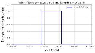
# start a new figure

figure()

# Plot the particle pass function versus z-velocity

plot(vz,particle_pass,"b-",label=' $R =$ %.2f mm'%R_mm)

xlim(min(vz),max(vz))

ylim(0.0,1.2)

xlabel(" $v_z$ [m/s]",fontsize=16)

ylabel("Transmitted truth value",fontsize=16)

grid(True)

title('Wien filter: $v =$ %.2e m, length $L =$ %.2f m'%(vmag,L))

legend(loc=1)

show()

# start a new figure

figure()

# Plot the particle pass function versus scaled z-velocity

plot(vz/vzpass,particle_pass,"b-",label=' $R =$ %.2f mm'%R_mm)

xlim(min(vz/vzpass),max(vz/vzpass))

ylim(0.0,1.2)

xlabel(" $v_z/v_{z,pass}$ ",fontsize=16)

ylabel("Transmitted truth value",fontsize=16)

grid(True)

legend(loc=1)

title('Wien filter: $v_{z,pass} =$ %.2e m, length $L =$ %.2f m'%(vzpass,L))

show()

Translations

Code	Language		Translator	Run

Credits

Fremont Teng; Loo Kang Wee; based on codes by E. Behringer

provided excerpts related to a set of exercises focused on the Wien (E x B) filter. Developed by E. Behringer, these exercises aim to guide students in understanding the behavior of charged particles moving through mutually perpendicular electric and magnetic fields. The ultimate goal is to simulate the operation of a Wien filter and analyze its velocity selection properties. The material is designed for first-year university physics students and beyond, with available implementation in Python.

2. Main Themes and Learning Objectives:

The core theme revolves around the interaction of charged particles with electromagnetic fields and how this interaction can be used for velocity selection. The exercises progressively build student understanding:

Force and Equations of Motion (Exercise 1): Students will learn to determine the Cartesian components of the forces acting on a charged particle in combined electric and magnetic fields and derive the corresponding equations of motion. The intro page explicitly states this learning objective: "generate equations predicting the Cartesian components of force acting on the charged particle and generate the equations of motion for the particle (Exercise 1)".
Trajectory Calculation and Visualization (Exercise 2): Students will utilize numerical integration to solve the derived equations of motion and calculate the trajectories of the charged particles. They will also learn to visualize these trajectories in both two and three dimensions. The learning objectives include: "calculate particle trajectories by solving the equations of motion (Exercise 2);" and "produce two-dimensional and three-dimensional plots of the trajectories (Exercise 2);". The description of the accompanying Python script, ExB_Filter_Exercise_3.py, confirms that it "is used to numerically integrate the second order linear differential equations that describe the trajectory of a charged particle through an E x B velocity filter."
Simulation of the Wien Filter (Exercise 3): The capstone of this set of exercises is the simulation of the Wien filter. Students will use their understanding and computational tools to model how the filter operates. The intro page highlights this as a key objective: "simulate the operation of an ( \vec{E} \times \vec{B} ) (Wien) filter (Exercise 3)".
Velocity Range and Geometry (Exercise 4 - implied): While not explicitly detailed in the excerpts, the learning objective mentions determining "the range of particle velocities transmitted by the filter, and how these are affected by the geometry of the filter (Exercise 4)." Exercise 3 likely lays the groundwork for this analysis.

3. Key Concepts and Principles:

Electromagnetic Force: The exercises are based on the Lorentz force law, which describes the force on a charged particle in the presence of electric and magnetic fields.
Equations of Motion: Applying Newton's second law (F=ma) to the electromagnetic force leads to the differential equations that govern the particle's motion.
Numerical Integration: Due to the complexity of the equations of motion in combined fields, numerical methods are employed to find the particle trajectories. The text explicitly mentions "numerical integration" in the intro page and the Python script.
Velocity Selection: A Wien filter utilizes perpendicular electric and magnetic fields to select particles with a specific velocity. At this specific velocity, the electric and magnetic forces balance, resulting in zero net force and no deflection. The text states, "Regions of mutually perpendicular electric and magnetic fields can be used to filter a collection of moving charged particles according to their velocity."
Pass Velocity: The excerpts define the specific velocity for which a particle experiences zero net force and passes undeflected through the filter: "( v_{pass} = - E_y / B_x )". This formula indicates that the pass velocity is determined by the magnitudes of the perpendicular electric field (in the y-direction) and magnetic field (in the x-direction).

4. Exercise 3 Details and Questions:

Exercise 3, supported by the ExB_Filter_Exercise_3.py script, focuses on simulating the filter's operation. The setup assumes:

The filter axis is aligned with the z-axis.
The magnetic field (( \vec{B} )) is in the +x direction (( B_x )).
The electric field (( \vec{E} )) is in the -y direction (( E_y )).

The exercise then poses questions related to the range of velocities transmitted by the filter through an exit aperture of radius ( R ) located at ( z = L ):

(a) Determine the maximum ( z )-velocity (( v_{z, max} = v_{pass} + \Delta v )) for which a ( Li^+ ) ion (assuming initial ( v_x = v_y = 0 )) will be transmitted through an aperture of radius ( R = 1.0 ) mm. What is the value of ( \Delta v / v_{pass} )?

(b) Repeat part (a) for an aperture of radius ( R = 2.0 ) mm and determine the new value of ( \Delta v / v_{pass} ).

These questions require the student to use the provided Python script (or their equivalent implementation from Exercise 2) to simulate the trajectories of ( Li^+ ) ions with varying initial ( z )-velocities around the calculated ( v_{pass} ). By observing which trajectories pass through the aperture at ( z = L ), they can determine the range of transmissible velocities and subsequently calculate ( \Delta v ) and ( \Delta v / v_{pass} ).

5. Relevant Code Snippets and Parameters:

The Python script ExB_Filter_Exercise_3.py provides several key parameters and functionalities:

Field Strengths:Ex = 0.0 # Ex = electric field in the +x direction [V/m]
Ey = -100.0 # Ey = electric field in the -y direction [V/m]
Ez = 0.0 # Ez = electric field in the +z direction [V/m]
Bx = 0.002 # Bx = magnetic field in the +x direction [T]
By = 0.0 # By = magnetic field in the +x direction [T]
Bz = 0.0 # Bz = magnetic field in the +x direction [T]
Aperture and Filter Dimensions:R_mm = 1.0 # R = radius of the exit aperture [mm]
L = 0.25 # L = length of the crossed field region [mm]
Particle Properties: The script includes placeholders for charge (( q )) and mass (( m )), and allows setting kinetic energy (KE_eV). For ( Li^+ ), these values would need to be defined.
Numerical Integration Setup: The script sets up the time interval for integration (tmax = L/vzpass), the number of time steps (N = 1000), and the time step size (h).
Derivatives Function: The derivs(r, t) function calculates the time derivatives of the particle's position and velocity based on the electromagnetic forces.
def derivs(r,t):
# derivatives of position components
xp = r[1]
yp = r[3]
zp = r[5]
dx = xp
dy = yp
dz = zp
# derivatives of velocity components
ddx = qoverm*(Ex + yp*Bz - zp*By)
ddy = qoverm*(Ey + zp*Bx - xp*Bz)
ddz = qoverm*(Ez + xp*By - yp*Bx)
return array([dx,ddx,dy,ddy,dz,ddz],float)
Velocity Scan: The script iterates over a range of initial ( z )-velocities around ( v_{pass} ) to determine which particles pass through the aperture.
vzpass = -Ey/Bx # z-velocity for zero deflection [m/s]
# Set up the array of z-velocities to try
vz = vzpass + linspace(-0.25*vzpass,0.25*vzpass,Ntraj+1) # the set of initial z-velocities
Output: The script includes a section to print the ( \Delta v ) and ( \Delta v / v_{pass} ) values when a change in the particle_pass array indicates the edge of the transmitted velocity range.

6. Conclusion:

The provided materials outline a comprehensive set of exercises designed to teach students about the principles and applications of the Wien (E x B) filter. By combining theoretical understanding with numerical simulations using Python, students will gain practical experience in analyzing the motion of charged particles in electromagnetic fields and the velocity selection capabilities of this important device. Exercise 3 specifically tasks students with quantifying the velocity range transmitted by the filter for different aperture sizes

Wien Filter Study Guide

Key Concepts

Wien Filter: A device that uses mutually perpendicular electric and magnetic fields to select charged particles based on their velocity.
Electric Force: The force experienced by a charged particle in an electric field, given by $\vec{F}_E = q\vec{E}$ , where $q$ is the charge and $\vec{E}$ is the electric field.
Magnetic Force (Lorentz Force): The force experienced by a moving charged particle in a magnetic field, given by $\vec{F}_B = q(\vec{v} \times \vec{B})$ , where $q$ is the charge, $\vec{v}$ is the velocity, and $\vec{B}$ is the magnetic field.
Equations of Motion: Mathematical expressions describing how the position of a particle changes over time, derived from Newton's second law ( $\vec{F} = m\vec{a}$ ). In this context, they involve the electric and magnetic forces.
Numerical Integration: A method for approximating the solution to differential equations, such as the equations of motion, by using discrete time steps.
Particle Trajectory: The path followed by a charged particle as it moves through space under the influence of forces.
Velocity Selector: A configuration of electric and magnetic fields where only particles with a specific velocity pass through undeflected.
Aperture: An opening that restricts which particles can pass through the Wien filter.
Transmitted Velocity Range: The range of velocities of particles that successfully pass through the Wien filter's aperture.

Quiz

Describe the configuration of the electric and magnetic fields in a Wien filter. How are they oriented with respect to each other?
For a charged particle moving through a Wien filter with a specific velocity, the net force is zero. Explain how the electric and magnetic forces balance each other in this scenario.
What are the learning objectives of the exercises associated with the Wien filter simulation described in the source material? List at least three objectives.
Explain the concept of a "pass velocity" ( $v_{pass}$ ) in the context of a Wien filter. How is it determined by the electric and magnetic field strengths?
Why is numerical integration necessary to find the trajectories of charged particles in a Wien filter for general cases? What kind of equations are being solved?
What factors determine whether a charged particle will pass through the exit aperture of a Wien filter in the simulation?
In the provided Python code excerpt, what is the purpose of the loop iterating through different values of vz? What physical quantity is being varied?
Explain the significance of the particle_pass array in the Python code. What does a value of 1 or 0 likely represent in this array?
How does the radius of the exit aperture affect the range of velocities of particles that can be transmitted by the Wien filter?
What does the term "charge to mass ratio" (qoverm) represent, and why is it an important parameter in analyzing the motion of charged particles in electromagnetic fields?

Quiz Answer Key

In a Wien filter, the electric field ( $\vec{E}$ ) and the magnetic field ( $\vec{B}$ ) are oriented such that they are mutually perpendicular to each other. Typically, if the particle is intended to move along the z-axis, the electric field might be in the y-direction and the magnetic field in the x-direction (or vice versa).
For a particle with the pass velocity, the electric force ( $\vec{F}_E = q\vec{E}$ ) and the magnetic force ( $\vec{F}_B = q(\vec{v} \times \vec{B})$ ) are equal in magnitude and opposite in direction. This results in a net force of zero on the particle, allowing it to pass through undeflected.
The learning objectives include generating equations of force and motion, calculating particle trajectories by solving these equations, producing plots of the trajectories in 2D and 3D, and simulating the operation of the Wien filter to determine the transmitted velocity range and its dependence on filter geometry.
The pass velocity ( $v_{pass}$ ) is the specific velocity at which a charged particle experiences zero net force in the Wien filter's crossed electric and magnetic fields and thus moves undeflected. It is given by the relationship $v_{pass} = -E_y / B_x$ (assuming $\vec{E} = (0, E_y, 0)$ and $\vec{B} = (B_x, 0, 0)$ and motion along the z-axis).
Numerical integration is needed because the equations of motion for a charged particle in combined electric and magnetic fields are often complex differential equations that do not have simple analytical solutions for arbitrary field configurations or initial conditions. Methods like numerical integration provide approximate solutions by breaking the motion into small time steps.
Whether a charged particle passes through the exit aperture depends on its trajectory as it moves through the region of the crossed fields. If the particle's deflection in the x-y plane at the exit ( $z=L$ ) is within the radius of the aperture, it will be transmitted; otherwise, it will be blocked.
The loop iterating through different values of vz in the Python code aims to simulate the behavior of particles entering the Wien filter with a range of initial velocities along the z-axis. By varying this initial velocity, the simulation determines which velocity ranges result in the particles passing through the filter's aperture.
The particle_pass array likely stores information about whether a particle with a particular initial z-velocity successfully passed through the exit aperture. A value of 1 could indicate that the particle passed, meaning its deflection was within the aperture radius, while a value of 0 could indicate that it was blocked.
A larger radius of the exit aperture allows a wider range of particle trajectories to be considered as "passing" through the filter. This generally leads to a broader range of transmitted velocities, as particles with slightly different initial velocities might still fall within a larger opening.
The charge to mass ratio ( $q/m$ ) is the ratio of a particle's electric charge to its mass. It is crucial because the acceleration of a charged particle in an electromagnetic field is directly proportional to this ratio ( $\vec{a} = (q/m)(\vec{E} + \vec{v} \times \vec{B})$ ). Therefore, particles with different $q/m$ values will experience different accelerations and follow different trajectories even with the same initial conditions and fields.

Essay Format Questions

Discuss the principles of operation of a Wien filter, explaining how the mutually perpendicular electric and magnetic fields are used to select charged particles based on their velocity. Analyze the conditions under which a particle passes through the filter undeflected.
Explain the process of simulating the behavior of charged particles in a Wien filter using numerical methods. Describe the key steps involved, including setting up the equations of motion, choosing a numerical integration technique, and determining if a particle is transmitted by the filter.
Analyze how the physical parameters of a Wien filter, such as the strengths of the electric and magnetic fields and the geometry of the filter (e.g., length of the field region, radius of the exit aperture), affect its performance as a velocity selector. Consider factors like the pass velocity and the transmitted velocity range.
Based on the provided source material, discuss the learning objectives of the Wien filter exercises. How do the different exercises (e.g., generating equations, calculating trajectories, simulating the filter) contribute to a student's understanding of electromagnetism and charged particle motion?
Consider the applications of Wien filters in scientific instruments and technologies. Research and discuss at least two real-world examples where Wien filters or similar velocity selection techniques are employed, explaining the specific purpose and advantages in each application.

Glossary of Key Terms

Cartesian Components: The components of a vector (like force or velocity) along the x, y, and z axes in a three-dimensional Cartesian coordinate system.
Charged Particle: A subatomic particle (like an electron or ion) that carries an electric charge.
Electric Field ( $\vec{E}$ ): A region of space around an electrically charged particle or object where a force would be exerted on other electrically charged particles or objects. Measured in units of Volts per meter (V/m) or Newtons per Coulomb (N/C).
Magnetic Field ( $\vec{B}$ ): A region of space around a magnet or moving electric charge in which a magnetic force would be exerted on other moving electric charges. Measured in units of Tesla (T).
Numerical Integration (odeint): A specific function (odeint) likely referring to a routine for numerical integration of ordinary differential equations, commonly found in scientific computing libraries like SciPy in Python.
Open Educational Resources (OER): Teaching, learning, and research materials that are freely available online for anyone to use, adapt, and share.
Open Source Physics (OSP): A project and community focused on developing and disseminating open-source computational tools and resources for physics education.
Simulation Model: A computational representation of a real-world system (in this case, a Wien filter and the motion of charged particles within it) used to study its behavior under different conditions.
Trajectory: The path traced by a moving object (in this case, a charged particle) through space as a function of time.
Velocity ( $\vec{v}$ ): The rate of change of an object's position with respect to time, including both its speed and direction. Measured in meters per second (m/s).
$\vec{E} \times \vec{B}$ : The cross product of the electric field vector and the magnetic field vector. The direction of the resulting vector is perpendicular to both $\vec{E}$ and $\vec{B}$ , and its magnitude is proportional to the product of their magnitudes and the sine of the angle between them. In the context of the Lorentz force, the magnetic force depends on $\vec{v} \times \vec{B}$ .
Li+ Ion: A lithium atom that has lost one electron, resulting in a net positive charge

Sample Learning Goals

[text]

For Teachers

[text]

Research

[text]

Video

[text]

Version:

Other Resources

[text]

end faq

{accordionfaq faqid=accordion4 faqclass="lightnessfaq defaulticon headerbackground headerborder contentbackground contentborder round5"}

Questions & Answers about the Wien (E x B) Filter Simulation

1. What is the fundamental purpose of a Wien filter, and what physical principles does it utilize?

A Wien filter is designed to selectively filter charged particles based on their velocity. It achieves this by employing mutually perpendicular electric and magnetic fields in a specific spatial region. The principle of operation relies on the forces exerted by these fields on moving charged particles. The electric field applies a force proportional to the charge and field strength in one direction, while the magnetic field applies a force proportional to the charge, velocity, and magnetic field strength, and in a direction perpendicular to both the velocity and the magnetic field. By carefully balancing the strengths of these fields, only particles with a specific velocity will experience zero net force and pass through undeflected.

2. What are the key learning objectives for students engaging with the Wien filter exercises described?

Students who complete these exercises will learn to:

Determine the Cartesian components of the electric and magnetic forces acting on a charged particle in perpendicular fields.
Derive the equations of motion for a charged particle moving through these fields.
Calculate the trajectory of a charged particle by numerically solving its equations of motion.
Generate 2D and 3D plots to visualize these trajectories.
Simulate the operation of a Wien filter.
Identify the range of particle velocities that are transmitted by the filter.
Analyze how the filter's geometry affects the range of transmitted velocities.

3. How does a Wien filter achieve velocity selection for charged particles?

Velocity selection in a Wien filter occurs when the electric force ( $q\vec{E}$ ) on a charged particle is exactly balanced by the magnetic force ( $q\vec{v} \times \vec{B}$ ). For mutually perpendicular electric field ( $\vec{E}$ in the y-direction) and magnetic field ( $\vec{B}$ in the x-direction), a particle moving with a velocity $\vec{v}$ in the z-direction will experience an electric force in the y-direction ( $qE_y\hat{j}$ ) and a magnetic force in the negative y-direction ( $-qv_zB_x\hat{j}$ ). When these forces are equal in magnitude and opposite in direction ( $qE_y = qv_zB_x$ ), the net force in the y-direction is zero, and the particle passes through the filter undeflected. This occurs for particles with a specific velocity $v_{pass} = -E_y/B_x$ .

4. What is the significance of numerical integration in analyzing the behavior of charged particles in a Wien filter?

The equations of motion for a charged particle in a Wien filter, especially when considering particles with initial velocity components not perfectly aligned with the z-axis or when analyzing the transmission of particles with a range of velocities, can be complex and may not have simple analytical solutions. Numerical integration techniques are therefore essential to approximate the solutions to these differential equations. These methods allow for the calculation of the particle's position and velocity at discrete time steps, enabling the simulation and analysis of particle trajectories under the influence of the electric and magnetic fields.

5. What role does the exit aperture of the Wien filter play in determining the transmitted range of velocities?

The exit aperture, typically a small circular opening placed along the intended path of undeflected particles, defines the spatial tolerance for a particle to be considered "transmitted" by the filter. Particles with velocities slightly different from the ideal $v_{pass}$ will experience a net force and thus a deflection in the y-direction. If this deflection is large enough that the particle's trajectory at the exit plane falls outside the bounds of the aperture, the particle is considered blocked. Therefore, the size (radius) of the exit aperture directly influences the range of velocities that can pass through the filter. A larger aperture will allow particles with a wider range of velocities (and thus greater deflections) to be transmitted, resulting in a broader velocity selection. Conversely, a smaller aperture will lead to a narrower range of transmitted velocities, providing finer velocity selection.

6. How can the simulation model be used to determine the range of particle velocities transmitted by the Wien filter?

The simulation model works by launching a large number of charged particles with a distribution of initial z-velocities around the ideal passing velocity ( $v_{pass}$ ) and with initial x and y velocities typically set to zero in these exercises. For each particle, the equations of motion are numerically integrated as it travels through the region with perpendicular electric and magnetic fields. At the end of the field region (at $z=L$ ), the particle's x and y coordinates are checked against the dimensions of the exit aperture (radius $R$ ). If the particle's position falls within the aperture ( $\sqrt{x^2 + y^2} \le R$ ), it is considered transmitted. By tracking which initial z-velocities result in transmission, and by systematically varying the range of initial velocities, the simulation can map out the "particle pass function" – a plot of transmission probability (or a binary pass/fail) versus initial z-velocity. The width of the velocity range for which particles are transmitted defines the velocity resolution of the filter.

7. How is the effect of the filter's geometry, such as the length of the crossed field region and the size of the exit aperture, investigated using the simulation?

The simulation allows for the manipulation of various geometrical parameters of the Wien filter. For instance, the length of the crossed field region ( $L$ ) can be changed in the simulation code (e.g., by modifying the L variable). Similarly, the radius of the exit aperture ( $R$ ) can be adjusted (e.g., by changing R_mm). By running the simulation multiple times with different values for these parameters while keeping other factors constant (like the electric and magnetic field strengths, and the charge-to-mass ratio of the particle), the effect of each geometrical factor on the filter's performance can be studied. This includes analyzing how the transmitted velocity range and the resolution of the filter change with variations in $L$ and $R$ . For example, increasing the length of the filter might lead to greater deflection for off-velocity particles, potentially narrowing the transmitted velocity range for a given aperture size. Similarly, changing the aperture size directly impacts the accepted deflection and thus the range of transmitted velocities, as explored in Exercise 4a and 4b.

8. What are some of the specific parameters and initial conditions used in the provided Python code snippet for simulating a Wien filter with a Li+ ion?

The Python code snippet provided includes the following key parameters and initial conditions:

Electric Field: $E_x = 0.0$ , $E_y = 100.0$ (in V/m), $E_z = 0.0$ .
Magnetic Field: $B_x = 0.002$ (in T), $B_y = 0.0$ , $B_z = 0.0$ .
Charge to Mass Ratio: qoverm = q/m (in C/kg), where q is the charge of the Li+ ion and m is its mass. This would need to be defined elsewhere in the full code.
Kinetic Energy: KE = KE_eV*1.602e-19 (in Joules), based on KE_eV (in electron volts), which is not explicitly defined in this snippet but would be set for the simulation.
Exit Aperture Radius: R_mm = 1.0 or 2.0 (in mm), converted to meters as R = 0.001*R_mm.
Length of Crossed Field Region: L = 0.25 (in mm), converted to meters.
Initial Position: $x_0 = 0.0$ , $y_0 = 0.0$ , $z_0 = 0.0$ (in meters).
Initial Velocities (except z): $dxdt_0 = 0.0$ , $dydt_0 = 0.0$ (in m/s). The initial z-velocity $dzdt_0 = vz[i]$ is varied within a range around the ideal passing velocity $vzpass = -Ey/Bx$ to study the velocity selection. The range is set by vz = vzpass + linspace(-0.25*vzpass,0.25*vzpass,Ntraj+1), where Ntraj is the number of trajectories simulated (1000 in this case).
Simulation Time: The simulation runs from $t_1 = 0.0$ to $t_2 = tmax = L/vzpass$ , with N = 1000 time steps.

These parameters are used to define the forces acting on the Li+ ion and to numerically integrate its trajectory for different initial z-velocities, ultimately determining which velocities allow the ion to pass through the exit aperture.

0.5 1 1 1 1 1 1 1 1 1 1 Rating 0.50 (1 Vote)

Details: Written by Fremont; Parent Category: 05 Electricity and Magnetism; Category: 08 Electromagnetism; Published: 30 April 2018; Created: 30 April 2018; Last Updated: 22 March 2025; Hits: 4938

Breadcrumbs

PICUP Wien (E x B) Filter Exercise 3 JavaScript HTML5 Applet Simulation Model need odeint to work

About

Translations

Credits

Wien Filter Study Guide

Key Concepts

Quiz

Quiz Answer Key

Essay Format Questions

Glossary of Key Terms

Sample Learning Goals

For Teachers

Video

Version:

Other Resources

end faq

Questions & Answers about the Wien (E x B) Filter Simulation

1. What is the fundamental purpose of a Wien filter, and what physical principles does it utilize?

2. What are the key learning objectives for students engaging with the Wien filter exercises described?

3. How does a Wien filter achieve velocity selection for charged particles?

4. What is the significance of numerical integration in analyzing the behavior of charged particles in a Wien filter?

5. What role does the exit aperture of the Wien filter play in determining the transmitted range of velocities?

6. How can the simulation model be used to determine the range of particle velocities transmitted by the Wien filter?

7. How is the effect of the filter's geometry, such as the length of the crossed field region and the size of the exit aperture, investigated using the simulation?

8. What are some of the specific parameters and initial conditions used in the provided Python code snippet for simulating a Wien filter with a Li+ ion?