About

"Derivative machine"

At the left side of the window one of 8 different predefined base functions y = f(x) can be selected by radio buttons. A suitable x range is attributed to each of them.

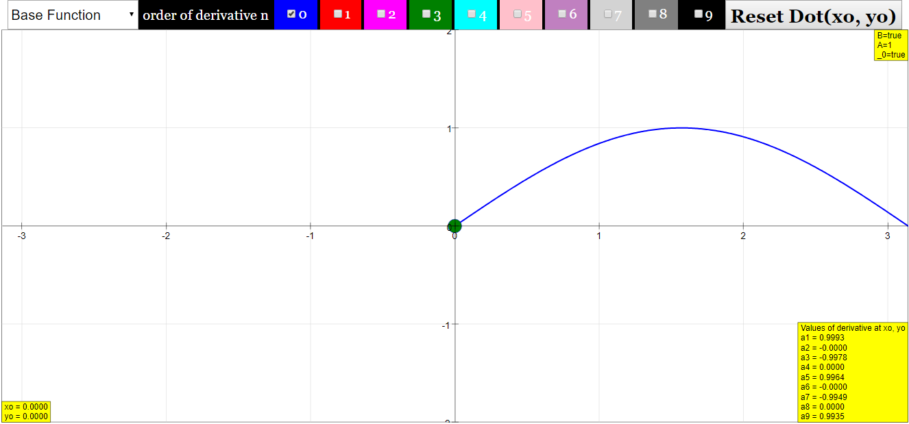
• Gaussian:  exp (-(x-3)²)
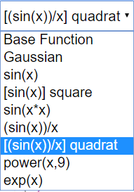
• sine (x)
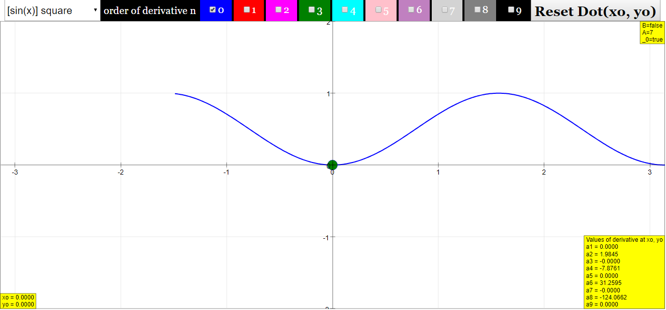
• (sine (x))²
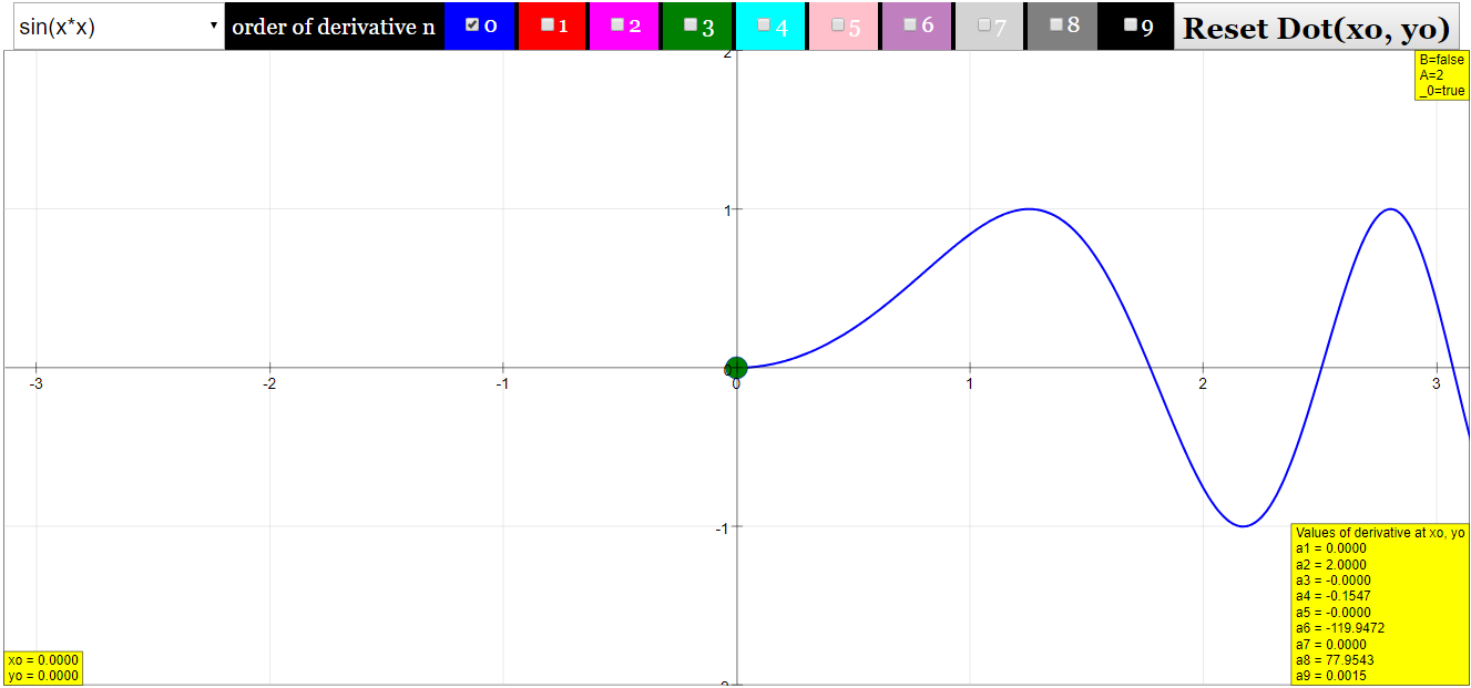
• sine (x²)
• (sine (x-20))/(x-20)
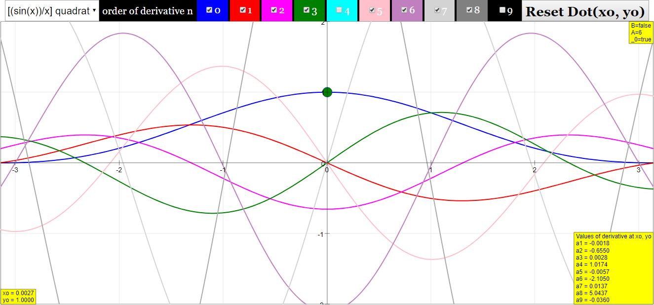
• [(sine (x-20))/(x-20)]²
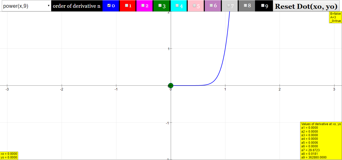
• Power function: pow (x,9) = x⁹ =x*x*x*x*x*x*x*x*x
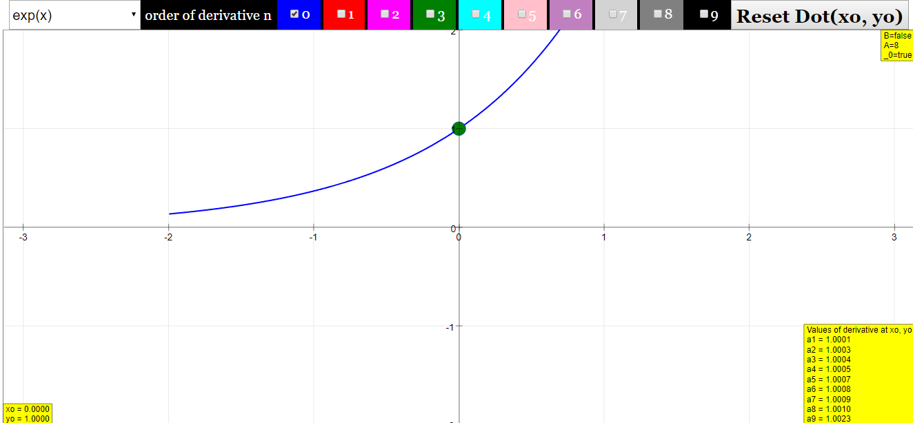
• Exponential: exp(x)

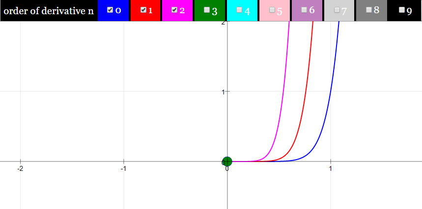
When the simulation is opened, the Gaussian function will be active. It is drawn as a blue curve. The zero line is shown in black.

At the top of the window there are 10 checkboxes to select derivatives of the base function. These are drawn as curves in the color of the check box numbers. Derivatives of different order can be shown simultaneously. Not all may be distinctly visible if their scales differ significantly. The scaling of the ordinate is self adjusting to the highest value.

A red dot on the curve defines a model point x₀, y₀ , for which the values of the derivatives a1 to a9 are shown in the number fields at the lower left. The dot can be drawn with the mouse to calculate derivatives for arbitrary model points. If it is drawn out of the abscissa range, it can be reset with the Reset Button.

Any one of the predefined functions can be selected with the Radio Buttons at the left.

For the sine function the curves of the 4^th and the 8^th derivative correctly coincide with that of the base function. The ninth derivative does not yet show visible irregularities by calculation or approximation errors.

With the power function, the 9^th derivative is a very high constant. At high x values the limited resolution of the difference algorithm results in increasing noise-like deviations.

The functions in this simulation are not editable as in other simulations of this course. The reason is that this is the only way the results for high order derivatives can be calculated real time. If you want to investigate other functions, open the simulation with the EJS Console, and change or add the simple code for a predefined function.

Derivatives

This simulation calculates a base function

y = f(x)

for 1000 x- values in a given interval.

With h the difference between consecutive x values sufficiently small, the first derivative (differential quotient) is approximated by the difference quotient

y⁽¹⁾(x) = (1/2h) [y(x+h) - y(x-h)]

The second derivative is approximated as the difference quotient of the first difference quotient

y⁽²⁾(x)= (1/2h) [y⁽¹⁾(x+h) - y⁽¹⁾(x-h)] = (1/2h)² [y(x+2h) - 2y(x) + y(x-1h)]

This algorithm can be continued, leading to the code lines for the base function a[0] and the derivatives up to the 9th order a[9].

For the predefined functions and intervals most approximations do not visually differ from the analytical derivatives. This can be best controlled with the sine function, where the derivatives look the same at every 4^th order.

For still higher derivatives, the limits of the accuracy of the approximation and also the computing accuracy are stressed, and noisy artifacts appear.

Code: With s = 1/(2h)

a0[j]=Math.pow(s,0)*y[0][j];

a1[j]=Math.pow(s,1)*(y2[1][j]-y1[1][j]);

a2[j]=Math.pow(s,2)*(y2[2][j]-2*y2[0][j]+y1[2][j]);

a3[j]=Math.pow(s,3)*(y2[3][j]-3*y2[1][j]+3*y1[1][j]-y1[3][j]);

a4[j]=Math.pow(s,4)*(y2[4][j]-4*y2[2][j]+6*y2[0][j]-4*y1[2][j]+y1[4][j]);

a5[j]=Math.pow(s,5)*(y2[5][j]-5*y2[3][j]+10*y2[1][j]-10*y1[1][j]+5*y1[3][j]-y1[5][j]);

a6[j]=Math.pow(s,6)*(y2[6][j]-6*y2[4][j]+15*y2[2][j]-20*y2[0][j]+15*y1[2][j]-6*y1[4][j]+y1[6][j]);

a7[j]=Math.pow(s,7)*(y2[7][j]-7*y2[5][j]+21*y2[3][j]-35*y2[1][j]+35*y1[1][j]-21*y1[3][j]+7*y1[5][j]-y1[7][j]);

a8[j]=Math.pow(s,8)*(y2[8][j]-8*y2[6][j]+28*y2[4][j]-56*y2[2][j]+70*y2[0][j]-56*y1[2][j]+28*y1[4][j]-8*y1[6][j]+y1[8][j]);

a9[j]=Math.pow(s,9)*(y2[9][j]-9*y2[7][j]+36*y2[5][j]-84*y2[3][j]+126*y2[1][j]-126*y1[1][j]+84*y1[3][j]-36*y1[5][j]+9*y1[7][j]-y1[9][j]);

The integers in the formulas follow simple generation rules, so that the series can be easily generated or continued.

E1:

• The first derivative describes the local steepness of the function´s curve
• The second derivative describes the local change of its steepness = curvature
• The third derivative describes the local change of its curvature =  ?
• The fourth derivative describes the local change in the change of curvature or the curvature of the curvature of the base function = ??
• ...and so on

Try to understand what the higher derivatives mean, as applied to the base curve of a function

E2:  Do the same for the sine function. Why does the 4^th derivative look like the base function? (Hint:  reason first why the second derivative looks like the negative of the base function, and then apply the same reasoning to the fourth and second derivative).

E3:  Go through the derivatives of the power function:  What type of parabola is each one?

(Hint:  the easy way is to reason downward from the 9th one).

E4:  Choose sine(x²). Consider why the derivatives assume higher and higher values (observe that the y scale is self adjusting!). Why are discernable oscillations shifting to higher x values with increasing order?

E5:  With sine(x)/x many derivatives are within comparable amplitude range, while looking quite different. Go through exercise E1 to understand the change in the basic function expressed by the different derivatives.

(Hint:  start by comparing any two consecutive derivatives)

 

Translations

Code	Language		Translator	Run

Credits

Dieter Roess; Fremont Teng; Loo Kang Wee

1. Introduction

This briefing document provides an overview of the "Derivative Machine JavaScript Simulation Applet HTML5," an open educational resource from Open Source Physics @ Singapore. This resource is designed to aid in learning and teaching calculus, specifically the concept of derivatives, through an interactive JavaScript simulation. The document outlines the main features, functionalities, underlying algorithm, suggested experiments, and pedagogical applications of the applet.

2. Main Themes and Important Ideas/Facts

The central theme of this resource is to provide a visual and interactive way for users to understand the concept of derivatives of a function, up to the ninth order. Key aspects and ideas highlighted in the description include:

• Interactive Visualization of Derivatives: The applet allows users to select a base function from eight predefined options and simultaneously visualize its derivatives up to the ninth order. These are displayed as colored curves alongside the base function (blue curve) and the zero line (black).
• "At the top of the window there are 10 checkboxes to select derivatives of the base function. These are drawn as curves in the color of the check box numbers. Derivatives of different order can be shown simultaneously."
• Exploration of Different Base Functions: Users can choose from a variety of functions using radio buttons, each with a suitable predefined x-range. The available functions are: Gaussian, sine(x), (sine(x))^2, sine(x^2), (sine(x-20))/(x-20), [(sine(x-20))/(x-20)]^2, Power function (x^9), and Exponential (exp(x)).
• "At the left side of the window one of 8 different predefined base functions y = f(x) can be selected by radio buttons."
• Dynamic Point for Derivative Evaluation: A movable red dot on the base function curve allows users to explore the values of the derivatives at any given x-value within the defined range. The corresponding derivative values (a1 to a9) are displayed in number fields.
• "A red dot on the curve defines a model point x0, y0, for which the values of the derivatives a1 to a9 are shown in the number fields at the lower left. The dot can be drawn with the mouse to calculate derivatives for arbitrary model points."
• Real-Time Calculation: The simulation calculates the derivatives in real-time, which is the reason why the base functions are not editable directly within the main applet.
• "The functions in this simulation are not editable as in other simulations of this course. The reason is that this is the only way the results for high order derivatives can be calculated real time."
• Numerical Approximation of Derivatives: The applet uses a finite difference algorithm to approximate the derivatives. The first derivative is approximated by the symmetric difference quotient: y(1)(x) = (1/2h) [y(x+h) - y(x-h)]. Higher-order derivatives are calculated iteratively as the difference quotient of the previous derivative.
• "With h the difference between consecutive x values sufficiently small, the first derivative (differential quotient) is approximated by the difference quotient y(1) (x) = (1/2h) [y(x+h) - y(x-h)]"
• Accuracy and Limitations: The resource acknowledges that the numerical approximation has limitations, especially for higher-order derivatives, where accuracy and computational precision can lead to "noisy artifacts." The sine function is presented as a good example to control the visual accuracy, as its derivatives repeat every fourth order. The power function demonstrates limitations at high x values due to the resolution of the algorithm.
• "For still higher derivatives, the limits of the accuracy of the approximation and also the computing accuracy are stressed, and noisy artifacts appear." "For the sine function the curves of the 4th and the 8th derivative correctly coincide with that of the base function. The ninth derivative does not yet show visible irregularities by calculation or approximation errors."
• Suggested Experiments (E1-E5): The resource includes several guided experiments designed to encourage deeper understanding of the meaning of higher-order derivatives, the properties of derivatives of specific functions (sine and power functions), and the behavior of derivatives for more complex functions like sine(x^2) and sine(x)/x.
• "E1: The first derivative describes the local steepness of the function´s curve The second derivative describes the local change of its steepness = curvature The third derivative describes the local change of its curvature = ?"
• Embeddability: The applet can be easily embedded into other webpages using an iframe code.
• "Embed this model in a webpage: "
• Customization via EJS Console: For users wanting to investigate other functions, the resource suggests opening the simulation with the EJS Console to modify or add code for predefined functions.
• "If you want to investigate other functions, open the simulation with the EJS Console, and change or add the simple code for a predefined function."
• Pedagogical Instructions: The "For Teachers" section provides instructions on how to use the different interactive elements of the applet, such as the function box, derivative checkboxes, and the reset dot button.

3. Potential Applications in Education

This simulation applet offers significant potential for educational applications in calculus and related mathematics courses:

• Visualizing Abstract Concepts: Derivatives, especially higher-order ones, can be abstract concepts. The applet provides a visual representation that can make these concepts more intuitive and understandable for students.
• Interactive Learning: The ability to select functions, view their derivatives simultaneously, and explore derivative values at different points through the movable red dot promotes active and interactive learning.
• Guided Exploration: The suggested experiments provide a structured approach for students to investigate the properties and meanings of derivatives for various types of functions.
• Understanding Limitations of Numerical Methods: The applet implicitly demonstrates the concept of numerical approximation and its limitations in terms of accuracy, especially for higher-order derivatives.
• Facilitating Discussions: The visual discrepancies and the results of the experiments can serve as excellent starting points for classroom discussions about the relationship between a function and its derivatives.
• Supplementary Learning Resource: This applet can be used as a supplementary resource alongside traditional calculus instruction, providing students with an additional tool for practice and conceptual understanding.

4. Conclusion

The "Derivative Machine JavaScript Simulation Applet HTML5" is a valuable open educational resource for teaching and learning calculus. Its interactive features, real-time calculations, and visual representations offer a powerful way to explore the concept of derivatives. The inclusion of suggested experiments and clear instructions further enhances its pedagogical value. While the numerical approximation method has inherent limitations for very high-order derivatives, the applet effectively demonstrates the fundamental concepts and relationships between a function and its lower-order derivatives for a variety of common functions.

Derivative Machine Simulation Study Guide

About the Simulation

The "Derivative Machine" is a JavaScript simulation applet designed to visually demonstrate the concept of derivatives for various base functions. Users can select from eight predefined functions and observe their derivatives up to the ninth order. The simulation approximates derivatives numerically using a finite difference method. A movable red dot allows users to explore the derivative values at specific points on the base function curve. The ordinate scaling automatically adjusts to display the highest value among the selected derivatives. The simulation is built using HTML5 and is part of the Open Educational Resources / Open Source Physics @ Singapore project.

Key Features of the Simulation

• Base Functions: Eight predefined functions are available for selection via radio buttons: Gaussian, sine(x), (sine(x))^2, sine(x^2), (sine(x-20))/(x-20), [(sine(x-20))/(x-20)]^2, power(x,9) = x^9, and exponential: exp(x).
• Derivatives: Ten checkboxes allow users to display derivatives from the 1st to the 9th order, along with the base function (0th order). Each derivative is plotted in a distinct color.
• Movable Point: A red dot on the base function curve can be dragged with the mouse. Number fields at the lower left display the values of the derivatives at the x-coordinate of this dot.
• Reset Button: This button resets the position of the red dot to its initial position if it is moved outside the abscissa range.
• Self-Adjusting Scale: The vertical axis (ordinate) automatically scales to accommodate the maximum value of the currently displayed derivatives.
• Real-time Calculation: Derivatives are calculated and displayed in real time as the user interacts with the simulation.

Mathematical Concepts

• Derivative: The derivative of a function measures the instantaneous rate of change of the function with respect to its variable. Geometrically, the first derivative at a point represents the slope of the tangent line to the curve at that point.
• Higher-Order Derivatives: Higher-order derivatives are obtained by repeatedly differentiating a function. The second derivative represents the rate of change of the first derivative (related to the concavity of the curve), the third derivative represents the rate of change of the second derivative (related to the rate of change of concavity), and so on.
• Difference Quotient: The simulation approximates derivatives using the difference quotient, a numerical method. The first derivative is approximated as (1/2h)[y(x+h) - y(x-h)], where h is a small difference between consecutive x values. Higher-order derivatives are calculated as the difference quotients of the lower-order difference quotients.
• Analytical vs. Numerical Derivatives: Analytical derivatives are found using the rules of calculus. Numerical derivatives are approximations obtained through methods like the difference quotient. The simulation demonstrates how numerical approximations can closely resemble analytical derivatives for sufficiently small h.

Experiments to Consider

• E1 (Interpretation of Higher Derivatives): Explore how each successive derivative relates to the shape and changes in the previous derivative's curve. Consider how steepness, curvature, and the rate of change of curvature are visually represented.
• E2 (Sine Function Derivatives): Observe the cyclical nature of the sine function's derivatives. Explain why the second derivative is the negative of the sine function and how this reasoning extends to the fourth derivative resembling the original function.
• E3 (Power Function Derivatives): Examine the shapes of the derivatives of the power function (x^9). Identify the type of polynomial (specifically, parabola or a related form) each derivative represents and how the degree of the polynomial changes with each differentiation.
• E4 (Sine(x^2) Derivatives): Analyze why the magnitudes of the derivatives of sine(x^2) increase with higher order. Investigate the reason behind the discernable oscillations shifting towards higher x values as the order of the derivative increases.
• E5 (Sine(x)/x Derivatives): Compare the shapes of the various derivatives of sine(x)/x, noting that their amplitudes remain relatively comparable. Relate the visual differences between consecutive derivatives to the concepts of steepness and changes in steepness.

Quiz

1. What are the eight predefined base functions available in the Derivative Machine simulation?
2. How does the simulation approximate the first derivative of a selected base function? Briefly describe the formula used.
3. Explain the purpose of the red dot on the curve and the number fields located at the lower left of the simulation window.
4. What happens to the scaling of the vertical axis (ordinate) when different derivatives are selected for display? Why is this feature useful?
5. For the sine(x) function, what is a notable observation about the relationship between the base function and its 4th and 8th derivatives?
6. Describe the behavior of the 9th derivative of the power function (x^9) as observed in the simulation, especially at higher x values.
7. Why are the base functions in this simulation not directly editable within the main applet window? What alternative is suggested for investigating other functions?
8. According to Experiment E1, what physical concept does the first derivative of a function's curve describe? What does the second derivative describe?
9. In Experiment E2, what hint is provided to help understand why the 4th derivative of sine(x) looks like the base function?
10. Briefly describe what happens to the oscillations of the derivatives of sine(x^2) as the order of the derivative increases, as highlighted in Experiment E4.

Answer Key

1. The eight predefined base functions are Gaussian (exp(-(x-3)^2)), sine(x), (sine(x))^2, sine(x^2), (sine(x-20))/(x-20), [(sine(x-20))/(x-20)]^2, power(x,9) = x^9, and exponential (exp(x)).
2. The simulation approximates the first derivative using the difference quotient formula: y'(x) ≈ (1/2h) [y(x+h) - y(x-h)], where h is a small difference between consecutive x values. This formula calculates the slope between two points close to x.
3. The red dot is a movable point on the base function's curve that the user can drag. The number fields at the lower left display the calculated values of the selected derivatives at the x-coordinate corresponding to the position of the red dot.
4. The ordinate scaling automatically adjusts to display the highest absolute value among the currently visible derivatives. This is useful because the magnitudes of different order derivatives can vary significantly, ensuring all selected curves are visible within the window.
5. For the sine(x) function, the simulation demonstrates that the curves of the 4th and the 8th derivatives correctly coincide with that of the base function, indicating a cyclical relationship.
6. The 9th derivative of the power function (x^9) is a very high constant. At high x values, the simulation shows increasing noise-like deviations due to the limited resolution of the difference algorithm.
7. The base functions are not editable in the main applet to allow for real-time calculation of high-order derivatives. The text suggests opening the simulation with the EJS Console to modify or add code for different predefined functions.
8. The first derivative describes the local steepness of the function's curve. The second derivative describes the local change of its steepness, which is also known as the curvature of the curve.
9. The hint in Experiment E2 suggests first reasoning why the second derivative of sine(x) looks like the negative of the base function (due to the changing slope), and then applying the same logic to the second derivative to understand the fourth derivative.
10. As the order of the derivative of sine(x^2) increases, the simulation shows that the discernable oscillations tend to shift towards higher x values, while the overall magnitude of the derivatives generally increases (as indicated by the self-adjusting y-scale).

Essay Format Questions

1. Discuss the relationship between a function and its first, second, and third derivatives. Using the "Derivative Machine" simulation, describe how these derivatives visually represent the rate of change, concavity, and the rate of change of concavity for a function of your choice.
2. Evaluate the effectiveness of the difference quotient method, as implemented in the "Derivative Machine," for approximating derivatives. Consider the trade-offs between accuracy and computational speed, and discuss any limitations or artifacts that might arise, particularly with higher-order derivatives or specific types of functions.
3. Choose two different base functions from the "Derivative Machine" simulation (e.g., sine(x) and power(x,9)). Compare and contrast the behavior of their derivatives up to the fourth order. Analyze the reasons for the observed similarities or differences in their graphical representations.
4. Explain how interactive simulations like the "Derivative Machine" can enhance the learning and teaching of calculus concepts, specifically the understanding of derivatives. Discuss the advantages of visual representation and hands-on exploration compared to traditional analytical methods alone.
5. Based on your exploration of the "Derivative Machine" and the experiments suggested, discuss the meaning and interpretation of higher-order derivatives (beyond the second derivative). How do they relate to the original function's properties, and what insights can they provide about its behavior?

Glossary of Key Terms

• Base Function: The original function, y = f(x), from which derivatives are calculated. In the simulation, users can select from eight predefined base functions.
• Derivative: A measure of how a function changes as its input changes. The first derivative represents the instantaneous rate of change or the slope of the tangent line.
• Higher-Order Derivative: The derivative of a derivative. The second derivative is the derivative of the first derivative, the third derivative is the derivative of the second derivative, and so on.
• Difference Quotient: A formula used to approximate the derivative of a function at a point using the values of the function at nearby points. It forms the basis of the numerical differentiation method used in the simulation.
• Abscissa: The horizontal coordinate (x-value) in a Cartesian coordinate system.
• Ordinate: The vertical coordinate (y-value) in a Cartesian coordinate system.
• Tangent Line: A straight line that touches a curve at a single point and has the same slope as the curve at that point (equal to the first derivative at that point).
• Curvature: The measure of how much a curve deviates from being a straight line. It is related to the second derivative of the function.
• Concavity: The direction in which a curve bends. A positive second derivative indicates the curve is concave up, and a negative second derivative indicates the curve is concave down.
• Algorithm: A step-by-step procedure for solving a problem or performing a computation. The simulation uses a specific algorithm based on the difference quotient to calculate derivatives.
• Real Time: Occurring instantaneously or with negligible delay, allowing for immediate feedback in response to user interaction.
• Self-Adjusting Scale: A feature where the axis limits of a graph automatically change to ensure all displayed data fits within the viewing area. In the simulation, the vertical axis scaling adjusts to the range of the displayed derivatives.

Sample Learning Goals

[text]

For Teachers

Derivative Machine JavaScript Simulation Applet HTML5

Instructions

Function Box

Order of Derivatives Check Boxes

Reset Dot Button

Toggling Full Screen

Research

[text]

Video

[text]

 Version:

Other Resources

[text]

What is the Derivative Machine JavaScript Simulation Applet?

The Derivative Machine is an interactive HTML5 simulation applet designed for learning and teaching calculus, specifically the concept of derivatives. It allows users to visualize a base function and up to its ninth derivative simultaneously.

How does the simulation work?

Users can select one of eight predefined base functions using radio buttons. Once a function is chosen, its graph (the zeroth derivative) is displayed. By toggling checkboxes, users can display higher-order derivatives of the selected function. A red dot on the curve allows users to explore the value of the function and its derivatives at a specific x-value, which is displayed in numerical fields. The simulation approximates the derivatives using a finite difference quotient algorithm.

What base functions are available in the simulation?

The simulation provides eight predefined base functions for exploration: Gaussian (exp(-(x-3)^2)), sine(x), (sine(x))^2, sine(x^2), (sine(x-20))/(x-20), [(sine(x-20))/(x-20)]^2, Power function (pow(x,9) = x^9), and Exponential (exp(x)). Each function has a suitable pre-set x-range.

How are the derivatives calculated in the simulation?

The simulation approximates derivatives numerically using the difference quotient method. For the first derivative, it uses y'(x) ≈ (1/2h) [y(x+h) - y(x-h)], where 'h' is a small difference between consecutive x values. Higher-order derivatives are calculated by applying the difference quotient to the previous derivative. For example, the second derivative is approximated as the difference quotient of the first difference quotient.

What can be learned by using this simulation?

Users can gain an intuitive understanding of the relationship between a function and its derivatives. They can observe how the first derivative relates to the slope of the original function, the second derivative relates to its curvature, and so on for higher orders. The simulation also allows exploration of how different base functions behave under differentiation and highlights concepts like periodicity in derivatives (e.g., with the sine function) and the potential for approximation errors at very high derivative orders.

How can the simulation be used for educational purposes?

The Derivative Machine can be used as a visual aid for teaching and learning calculus. Students can experiment with different functions and their derivatives, explore the meaning of higher-order derivatives, and observe the behavior of derivatives for various types of functions. Teachers can use it to illustrate key concepts and assign exercises based on the observations made using the simulation, such as analyzing the derivatives of sine, power, or composite functions.

What are the limitations of the simulation?

The simulation approximates derivatives numerically, which can lead to inaccuracies, especially for very high-order derivatives or at high x values for certain functions like the power function due to the limited resolution of the algorithm and computing accuracy. The predefined functions are not directly editable within the main applet interface to ensure real-time calculations for high-order derivatives. However, the source code can be modified using the EJS Console for those who want to investigate other functions.

How can I interact with the simulation?

Users can interact with the simulation by selecting a base function using the radio buttons on the left. They can then toggle the checkboxes at the top to display different orders of derivatives. By dragging the red dot on the graph, users can examine the values of the function and its derivatives at specific x-values shown in the number fields at the lower left. The "Reset Button" can be used to return the red dot to its initial position if it is dragged out of the visible range. Double-clicking the panel toggles full-screen mode.