About

Magnetic Field from Loops

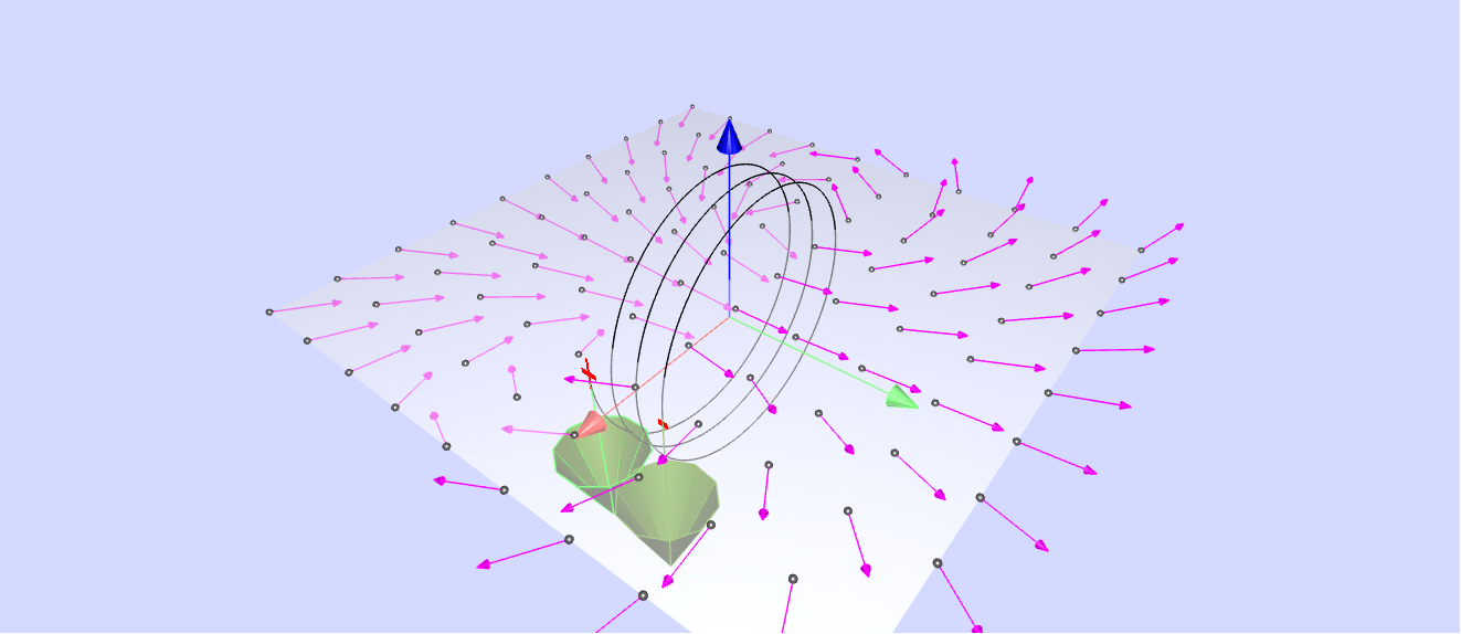
The EJSMagnetic Field from Loops model computes the B-field created by an electric current through a straight wire, a closed loop, and a solenoid. The user can adjust the vertical position of the slice through the 3D field.

1. Watch the simulation as the field changes from the field around a long straight current-carrying wire to the field near a coil. Explain what happens to the field. Inside a coil of many loops, why is the field fairly uniform near the center (think about vector addition and what vectors would be adding together near the center).
2. There is an arrow on each end of the wire (red and blue).  Which one shows the direction of the current in the wire? Explain.
3. The simulation also shows the magnetic flux. What is flux? Therefore, what do the different colors represent and why (i.e is pink higher flux than yellow or vice versa)? and what does "higher flux" mean in terms of the geometry and field strength?)?

Credits:

The Magnetic Field from Loops simulation was created by Fu-Kwun Hwang using the Easy Java Simulations (EJS) modeling tool and was adapted to EJS version 4.1 by Robert Mohr and Wolfgang Christian at Davidson College. Additional exercises written by Anne J. Cox. You can examine and modify the model for this simulation if you have Ejs installed by right-clicking within the simulation frame and selecting "Open Ejs Model" from the pop-up menu. Information about EJS is available at: <http://www.um.es/fem/Ejs/> and in the OSP ComPADRE collection <http://www.compadre.org/OSP/>.

 

Translations

Code	Language		Translator	Run

Credits

Fu-Kwun Hwang, Wolfgang Christian, Robert Mohr remixed by lookang (weelookang@gmail.com); Fremont Teng; Loo Kang Wee

Overview:

This document provides a review of the "Magnetic Field From Loop Simulator JavaScript Simulation Applet HTML5," an interactive simulation tool hosted on the Open Educational Resources / Open Source Physics @ Singapore website. This simulation is designed to help users visualize and understand the magnetic fields generated by electric currents in various configurations, including straight wires, closed loops, and solenoids. The document outlines the main features, educational objectives, and potential applications of this resource.

Main Themes and Important Ideas/Facts:

1. Visualization of Magnetic Fields: The primary focus of the simulation is to provide an interactive 3D visualization of magnetic fields created by electric currents. Users can rotate, zoom, and slice through the 3D representation to observe the field lines. This feature aims to make the abstract concept of magnetic fields more tangible and understandable. The website highlights this, stating: "Experience magnetic field lines like never before. Rotate, zoom, and slice through the 3D representation to uncover the intricate beauty of electromagnetic fields."
2. Exploration of Different Current Configurations: The simulator allows users to investigate the magnetic fields produced by:

• A long straight current-carrying wire.
• A closed loop of current.
• A solenoid (a coil of many loops). The "About" section explicitly mentions this capability: "The EJSMagnetic Field from Loops model computes the B-field created by an electric current through a straight wire, a closed loop, and a solenoid."

1. Adjustable Parameters for Deeper Understanding: The simulation offers several adjustable parameters that enable users to explore the relationships between current and the resulting magnetic field. These parameters include:

• Current intensity.
• Number of loops (relevant for coils and solenoids).
• Vertical position of the slice through the 3D field (Z-slice).
• Magnetic poles (North and South are visually represented). The description emphasizes this interactivity: "Adjustable Parameters for Deeper Insight Control every aspect of the simulation, including: * Current intensity * Number of loops * Z-slice for cross-sectional analysis * Magnetic poles (North and South)".

1. Learning Through Experimentation and Observation: The simulation is designed as an educational tool that encourages active learning. The "Learn Through Play" section suggests specific experiments:

• Applying the Right-Hand Grip Rule to understand the relationship between current direction and pole formation.
• Experimenting with multiple loops to observe the superposition of magnetic fields.
• Visualizing symmetry in 2D and 3D planes.

1. Understanding Magnetic Flux: The simulation also displays magnetic flux. Users are prompted to consider what flux is and how the different colors in the visualization represent varying levels of flux. The description poses the question: "The simulation also shows the magnetic flux. What is flux? Therefore, what do the different colors represent and why (i.e is pink higher flux than yellow or vice versa)? and what does 'higher flux' mean in terms of the geometry and field strength?)?" This encourages users to connect the visual representation with the theoretical concept of magnetic flux.
2. Uniform Field Inside a Solenoid: One of the suggested activities encourages users to explain why the magnetic field inside a coil of many loops is fairly uniform near the center. This prompts them to think about the vector addition of the magnetic fields from individual loops. The description asks: "Inside a coil of many loops, why is the field fairly uniform near the center (think about vector addition and what vectors would be adding together near the center)."
3. Direction of Current: The simulation uses colored arrows (red and blue) on the wire to indicate the direction of the current. Users are asked to identify which color represents the current direction and explain their reasoning. This reinforces the conventional representation of current direction. The description states: "There is an arrow on each end of the wire (red and blue). Which one shows the direction of the current in the wire? Explain."
4. Real-World Applications: The resource highlights the practical relevance of understanding magnetic fields, linking the simulation to applications such as:

• Electromagnets, motors, and transformers (which utilize solenoids).
• MRI machines.
• The Biot-Savart law. The "Applications in Real Life" section emphasizes this connection: "This simulation is not just academic—it’s practical. It helps to understand: * How solenoids are used in electromagnets, motors, and transformers. * The principles behind MRI machines and other electromagnetic devices. * The real-world applications of the Biot-Savart law."

1. Target Audience: The simulation is designed for a broad audience, including students, teachers, and science enthusiasts. It aims to make the learning of electromagnetism more accessible and engaging. The "Why It’s Perfect for You" section explicitly addresses these groups.
2. Technical Details and Credits: The simulation was created using Easy Java Simulations (EJS) and adapted for web use (webEJS and EJS version 4.1). Credits are given to Fu-Kwun Hwang, Wolfgang Christian, Robert Mohr, lookang, Fremont Teng, and Loo Kang Wee for their contributions. The page also provides information on accessing and modifying the model with EJS.

Key Quotes:

• "The EJSMagnetic Field from Loops model computes the B-field created by an electric current through a straight wire, a closed loop, and a solenoid." (About section)
• "Watch the simulation as the field changes from the field around a long straight current-carrying wire to the field near a coil. Explain what happens to the field." (Exercise 1)
• "Inside a coil of many loops, why is the field fairly uniform near the center (think about vector addition and what vectors would be adding together near the center)." (Exercise 1)
• "There is an arrow on each end of the wire (red and blue). Which one shows the direction of the current in the wire? Explain." (Exercise 2)
• "The simulation also shows the magnetic flux. What is flux? Therefore, what do the different colors represent and why (i.e is pink higher flux than yellow or vice versa)? and what does 'higher flux' mean in terms of the geometry and field strength?)?" (Exercise 3)
• "Experience magnetic field lines like never before. Rotate, zoom, and slice through the 3D representation to uncover the intricate beauty of electromagnetic fields." (Interactive 3D Visualization)
• "Adjustable Parameters for Deeper Insight Control every aspect of the simulation, including: * Current intensity * Number of loops * Z-slice for cross-sectional analysis * Magnetic poles (North and South)" (Adjustable Parameters for Deeper Insight)
• "Apply the Right-Hand Grip Rule to see how current direction influences pole formation." (Learn Through Play)
• "This simulation is not just academic—it’s practical. It helps to understand: * How solenoids are used in electromagnets, motors, and transformers. * The principles behind MRI machines and other electromagnetic devices. * The real-world applications of the Biot-Savart law." (Applications in Real Life)

Conclusion:

The "Magnetic Field From Loop Simulator JavaScript Simulation Applet HTML5" is a valuable educational resource for understanding the principles of electromagnetism. Its interactive 3D visualizations, adjustable parameters, and guided questions facilitate a deeper and more intuitive grasp of magnetic fields generated by various current configurations. By connecting theoretical concepts with visual representations and real-world applications, this simulation serves as an effective tool for students, teachers, and anyone interested in exploring the fascinating world of electromagnetism. The availability as an open educational resource further enhances its accessibility and potential impact.

 

Study Guide: Magnetic Field from Current Loops Simulation

Key Concepts

• Magnetic Field (B-field): The region around a magnet or a current-carrying conductor where a magnetic force is exerted. It is a vector quantity, having both magnitude and direction.
• Current-Carrying Wire: An electrical conductor through which electric current flows, generating a magnetic field around it.
• Magnetic Field Lines: Imaginary lines that represent the direction and strength of a magnetic field. The density of the lines indicates the field strength, and the tangent to the lines indicates the field direction.
• Right-Hand Grip Rule: A mnemonic used to determine the direction of the magnetic field around a current-carrying wire or the poles of a solenoid. For a straight wire, if the thumb points in the direction of the current, the fingers curl in the direction of the magnetic field. For a loop or solenoid, if the fingers curl in the direction of the current, the thumb points towards the North pole of the magnetic field.
• Magnetic Field from a Loop: A current-carrying loop of wire creates a magnetic field similar to that of a bar magnet, with a North and South pole. The field is stronger inside the loop.
• Solenoid: A coil of wire wound into a tightly packed helix. When current flows through it, a relatively uniform magnetic field is created inside the solenoid, and the field outside resembles that of a bar magnet.
• Vector Addition of Magnetic Fields: The total magnetic field at a point due to multiple current sources is the vector sum of the magnetic fields produced by each individual source at that point.
• Magnetic Flux (Φ): A measure of the total magnetic field that passes through a given area. It is defined as Φ = ∫ B ⋅ dA, where B is the magnetic field vector and dA is the area vector. In simpler terms, it represents the "amount" of magnetic field lines passing through a surface.
• Flux Density: The amount of magnetic flux per unit area, which is equivalent to the magnitude of the magnetic field (B). Higher flux density indicates a stronger magnetic field.

Quiz

1. Describe the change in the magnetic field as the simulation transitions from a long straight wire to a coil with multiple loops. What causes this transformation in the field pattern?
2. In the simulation, there are red and blue arrows at the ends of the wire. Identify which arrow indicates the direction of the current and explain the reasoning behind your choice based on the observed magnetic field direction.
3. Define magnetic flux in your own words. According to the simulation, what do the different colors representing magnetic flux likely indicate? Explain the relationship between color, flux intensity, and the underlying magnetic field strength and geometry.
4. Consider the magnetic field inside a coil of many loops, particularly near the center. Explain why this field is relatively uniform compared to the field near a single loop or the edges of the coil, referencing the principle of vector addition.
5. How does the simulation demonstrate the application of the right-hand grip rule? Describe a specific scenario within the simulation and how the rule can be used to predict the direction of the magnetic field or the poles of the electromagnet.
6. Explain how increasing the number of loops in the simulation affects the overall magnetic field strength, both inside and outside the coil. What fundamental principle of electromagnetism explains this effect?
7. What similarities can you observe between the magnetic field produced by a solenoid (a coil with many loops) in the simulation and the magnetic field of a permanent bar magnet? Identify at least one key difference.
8. The simulation allows for adjusting a "z-slice." Explain what this feature represents and how it aids in understanding the three-dimensional nature of the magnetic field produced by the current-carrying loops.
9. Describe a real-world application of solenoids mentioned in the text. How does the behavior of the magnetic field in the simulation help to understand the functionality of this application?
10. How can this interactive simulation be a more effective learning tool for understanding electromagnetism compared to static diagrams in a textbook? Provide at least two specific reasons based on the features described.

Answer Key

1. As the simulation transitions from a straight wire to a coil, the magnetic field lines begin to loop around each individual segment of the wire and, more significantly, become concentrated and more uniform inside the loop(s). This occurs because the magnetic fields generated by each segment of the wire in the loop add vectorially, resulting in a stronger and more directed field, especially in the interior.
2. The blue arrow typically shows the direction of the conventional current (positive charge flow). According to the right-hand grip rule, if you point your thumb in the direction of the blue arrow, your fingers will curl in the direction of the magnetic field lines shown in the simulation around a single wire segment.
3. Magnetic flux is the measure of the total magnetic field passing through a given area. Different colors in the simulation likely represent different intensities of magnetic flux. A color indicating "higher flux" (e.g., a more intense color) means that more magnetic field lines are passing through that area, implying a stronger magnetic field strength or a geometry where the field lines are more concentrated.
4. Near the center of a coil with many loops, the magnetic field vectors produced by each individual loop segment tend to point in roughly the same direction (along the axis of the coil). Through vector addition, these individual contributions reinforce each other, resulting in a relatively strong and uniform field directed along the axis. The perpendicular components of the fields from different segments tend to cancel out near the center.
5. The simulation demonstrates the right-hand grip rule by visually showing the relationship between the direction of current in the wire (indicated by the arrows) and the resulting magnetic field lines (their direction and orientation). For example, observing a single loop, if you curl your fingers in the direction of the (blue) current arrow, your thumb will point towards the North pole of the magnetic field created by the loop, consistent with the simulation's depiction of field lines exiting that side.
6. Increasing the number of loops in the simulation significantly increases the overall magnetic field strength. This is because each loop carrying current generates its own magnetic field, and when these loops are arranged close together in a coil or solenoid, their magnetic fields add constructively (vectorially) in the interior, leading to a stronger combined field.
7. The magnetic field of a solenoid in the simulation exhibits a clear North and South pole, with field lines exiting the North pole and entering the South pole, similar to a bar magnet. The field is relatively uniform inside the solenoid, analogous to a (simplified) uniform field within an ideal bar magnet. A key difference is that the magnetic field of the solenoid is generated by electric current, whereas a permanent magnet's field originates from the intrinsic magnetic moments of its constituent atoms.
8. The "z-slice" represents a cross-sectional plane through the three-dimensional magnetic field distribution produced by the current loops. By adjusting the vertical position of this slice, users can observe the magnitude and direction of the magnetic field at different points along the axis perpendicular to the plane of the loops, providing a better understanding of the field's spatial variation.
9. The text mentions that solenoids are used in electromagnets, motors, and transformers. The simulation's depiction of a strong and controllable magnetic field generated by a current in a coil helps understand how electromagnets work (by turning the current on and off, the magnetic field can be controlled). This controllable magnetic field is also fundamental to the operation of electric motors and transformers, which rely on the interaction between magnetic fields and electric currents.
10. This interactive simulation is more effective because it provides a dynamic and visual representation of an abstract concept like the magnetic field. Users can actively manipulate parameters (current, number of loops, slice position) and observe the immediate effects on the field, fostering a deeper intuitive understanding compared to static images. The 3D visualization also allows for exploration of the field in space, which is difficult to grasp from two-dimensional diagrams alone.

Essay Format Questions

1. Discuss how the interactive simulation of magnetic fields from current loops effectively demonstrates the principles of electromagnetism, focusing on the relationship between electric current and the generation of magnetic fields.
2. Analyze the magnetic field patterns produced by a single current loop and a solenoid as depicted in the simulation. Compare and contrast these patterns and explain how the arrangement of multiple loops in a solenoid leads to a more uniform internal magnetic field.
3. Evaluate the role of the right-hand grip rule in understanding and predicting the direction of magnetic fields generated by current-carrying wires and loops, referencing specific observations you can make using the simulation.
4. Explain the concept of magnetic flux and how the simulation visually represents variations in flux density. Discuss the significance of magnetic flux in the context of electromagnetic induction (though not explicitly shown in this simulation).
5. Describe how simulations like the "Magnetic Field From Loop SImulator" can enhance the learning experience in physics education compared to traditional methods. Discuss the benefits of interactive visualization and experimentation in grasping abstract scientific concepts.

Glossary of Key Terms

• Electromagnetism: The branch of physics concerned with the forces that occur between electrically charged particles. It encompasses both electric and magnetic phenomena, which are fundamentally intertwined.
• Current Intensity: The magnitude of the electric current, typically measured in Amperes (A), representing the rate of flow of electric charge. In the simulation, adjusting this parameter affects the strength of the magnetic field.
• Number of Loops: The quantity of individual turns of wire in a coil or solenoid. Increasing the number of loops in a solenoid generally strengthens the magnetic field it produces.
• Z-slice: A cross-sectional plane perpendicular to the axis of the current loop(s), allowing visualization of the magnetic field at a specific vertical position in the simulation's 3D space.
• Magnetic Poles (North and South): Regions at opposite ends of a magnet where the magnetic field is strongest. Magnetic field lines emerge from the North pole and enter the South pole. Current loops and solenoids also exhibit magnetic poles.
• Superposition of Magnetic Fields: The principle that the total magnetic field at a point due to multiple current-carrying conductors or magnets is the vector sum of the individual magnetic fields produced by each source at that point.
• Biot-Savart Law: A fundamental law in electromagnetism that describes the magnetic field generated by a steady electric current. While not explicitly used in the simulation's interface, it is the underlying principle governing the calculated magnetic fields.

Explore Electromagnetism Like Never Before with Our Interactive Simulation!

---

Ever wondered how magnetic fields are created by electric currents? Dive into the fascinating world of electromagnetism with this visually stunning and highly interactive simulation of circular current loops. Whether you’re a student, teacher, or science enthusiast, this tool will electrify your understanding of magnetic fields and their behavior.

---

What Makes This Simulation Special?

💡 Interactive 3D Visualization

https://sg.iwant2study.org/ospsg/index.php/702 link

 

Experience magnetic field lines like never before. Rotate, zoom, and slice through the 3D representation to uncover the intricate beauty of electromagnetic fields.

🎚️ Adjustable Parameters for Deeper Insight
Control every aspect of the simulation, including:

• Current intensity
• Number of loops
• Z-slice for cross-sectional analysis
• Magnetic poles (North and South)

📈 Dynamic Graphs in Real-Time
Observe the magnetic field strength dynamically along the z-plane, helping you correlate theory with visuals.

---

Learn Through Play

This simulation is more than just a tool—it’s an educational playground:

• Apply the Right-Hand Grip Rule to see how current direction influences pole formation.
• Experiment with Multiple Loops to witness the superposition of magnetic fields.
• Visualize Symmetry in 2D and 3D planes for a comprehensive understanding.

---

Why It’s Perfect for You

• For Students: Struggling with electromagnetism concepts? This tool brings textbook diagrams to life, making complex ideas easy to grasp.
• For Teachers: Engage your students with a hands-on virtual lab experience. Perfect for in-class demonstrations or homework assignments.
• For Enthusiasts: Satisfy your curiosity about the physics of magnetic fields and solenoids.

---

How to Get Started

1. Visit the simulation here.
2. Adjust the sliders to experiment with current, loops, and z-slices.
3. Hit "Play" to watch the magic of electromagnetism in action!

📌 Pro Tip: Refresh your browser to reset and explore new configurations.

---

Applications in Real Life

This simulation is not just academic—it’s practical. It helps to understand:

• How solenoids are used in electromagnets, motors, and transformers.
• The principles behind MRI machines and other electromagnetic devices.
• The real-world applications of the Biot-Savart law.

---

Share and Inspire!

Tag your friends, colleagues, or students who love physics and engineering. Let’s make science accessible and engaging for everyone. Use the hashtag #MagneticFieldExplorer to join the conversation.

---

Closing Thoughts

This simulation is proof that learning science doesn’t have to be boring. With just a click, you can explore the invisible forces shaping our universe. So, why wait? Dive into this interactive world of magnetic fields and ignite your passion for physics today!

---

📢 Spread the Word!
Like it? Share it! Let’s inspire the next generation of physicists and engineers.

For Teachers

Magnetic Field From Loop SImulator JavaScript Simulation Applet HTML5

Instructions

Combo Box and Sliders

Toggling Full Screen

Play/Pause and Reset Buttons

Research

[text]

Video

[text]

 Version:

1. https://weelookang.blogspot.com/2025/01/explore-electromagnetism-like-never.html

Other Resources

[text]

Frequently Asked Questions: Magnetic Fields from Current Loops

1. How does the magnetic field change as a current-carrying straight wire is formed into a coil or solenoid, and why is the field uniform near the center of a long solenoid?

When a long straight current-carrying wire is formed into a loop, the magnetic field lines, which initially form concentric circles around the wire, begin to loop through the center of the newly formed loop. As more loops are added to create a coil or solenoid, the magnetic field lines from each individual loop begin to align and reinforce each other, particularly within the interior of the coil. Near the center of a long solenoid with many tightly packed loops, the magnetic field becomes fairly uniform. This uniformity arises due to vector addition. The magnetic field vectors produced by individual loops have components that are perpendicular to the axis of the solenoid and components that are parallel to the axis. Near the center, the perpendicular components from different loops largely cancel each other out due to symmetry, while the parallel components add together constructively, resulting in a strong and relatively uniform magnetic field directed along the axis of the solenoid.

2. The simulation shows red and blue arrows on the ends of the wire. Which color represents the direction of the current, and how can you determine this?

The simulation, when used in conjunction with the right-hand grip rule, allows you to determine the direction of the current. Conventionally, if you curl the fingers of your right hand in the direction of the current flow in the loop (from positive to negative), your thumb will point in the direction of the magnetic field inside the loop (the North pole). The red and blue arrows likely represent the direction of the current and the resulting magnetic poles. By observing the direction that would produce the depicted magnetic field lines according to the right-hand rule, you can infer which color corresponds to the current direction. Typically, one color might represent the conventional current direction, while the other might implicitly indicate the electron flow or be related to the resulting magnetic poles (e.g., one end acting as a North pole and the other as a South pole due to the current).

3. The simulation displays magnetic flux with different colors. What is magnetic flux, and what do the different colors signify in terms of flux strength and its relation to geometry and field strength?

Magnetic flux ($\Phi_B$) is a measure of the total magnetic field that passes through a given area. Quantitatively, it is the product of the magnetic field strength (B), the area (A) through which it passes, and the cosine of the angle ($\theta$) between the magnetic field vector and the normal to the surface ($\Phi_B = BA\cos\theta$). Therefore, magnetic flux is highest when the magnetic field is strong, the area through which it passes is large, and the magnetic field is perpendicular to the surface. In the simulation, different colors likely represent varying magnitudes of magnetic flux. For instance, one color (e.g., pink) might indicate a region of higher magnetic flux, meaning that either the magnetic field strength is greater in that area, or the field lines are more concentrated (passing through a given area), or the orientation is more perpendicular to the surface being considered. Conversely, another color (e.g., yellow) might represent lower magnetic flux. "Higher flux" geometrically implies a greater density of magnetic field lines passing through a given surface and corresponds to a stronger overall magnetic effect in that region.

4. What is the right-hand grip rule, and how can it be applied using this simulation?

The right-hand grip rule is a mnemonic used to determine the direction of the magnetic field produced by a current-carrying wire or the direction of the force on a moving charge in a magnetic field. For a current loop, if you curl the fingers of your right hand in the direction of the conventional current flow (positive to negative), your thumb will point in the direction of the magnetic field lines inside the loop, which is also the direction of the North magnetic pole. The simulation allows you to visualize the magnetic field lines produced by different configurations of current-carrying wires (straight, loop, solenoid). By observing the direction of the current (inferred from the simulation's representation) and then applying the right-hand grip rule, you can predict the direction of the resulting magnetic field and verify it with the simulation's visual output. Conversely, you can use the observed magnetic field direction to deduce the direction of the current.

5. How can you experiment with multiple loops in the simulation, and what does this demonstrate about the superposition of magnetic fields?

The simulation provides controls, likely sliders or input fields, to adjust the number of loops in a coil or solenoid. By increasing the number of loops while keeping other parameters (like current intensity) constant, you can observe how the overall magnetic field changes. This demonstrates the principle of superposition for magnetic fields. The magnetic field at any point due to multiple current sources is the vector sum of the magnetic fields that would be produced by each source individually. When you add more loops to a coil, the magnetic field produced by each loop contributes to the total field. Inside the coil, these contributions largely add up in the same direction along the axis, resulting in a stronger overall magnetic field proportional (ideally) to the number of loops. The simulation visually shows the increased density of magnetic field lines and the enhanced field strength as more loops are added, illustrating this superposition.

6. What real-world applications are related to the principles demonstrated by this simulation of magnetic fields from current loops and solenoids?

The principles demonstrated by this simulation are fundamental to numerous real-world technologies and phenomena. Solenoids, which are coils of wire, are used extensively as electromagnets in devices like electric motors (where the magnetic field from a solenoid interacts with permanent magnets to produce rotation), transformers (where changing magnetic fields in one coil induce currents in another), relays (electrically controlled switches), and actuators. The understanding of magnetic fields from loops is also crucial for technologies like Magnetic Resonance Imaging (MRI) machines, which use strong, uniform magnetic fields created by large superconducting solenoids to produce detailed images of the inside of the human body. Furthermore, the Biot-Savart law, which governs the magnetic field generated by an electric current, underlies the operation of many electromagnetic devices and is essential for designing and understanding them.

7. How can students and teachers benefit from using this interactive simulation?

This interactive simulation offers significant benefits for both students and teachers. For students, it provides a visual and hands-on way to explore abstract concepts in electromagnetism, such as magnetic fields, magnetic flux, and the right-hand rule. By adjusting parameters like current intensity and the number of loops and observing the real-time changes in the magnetic field, students can develop a more intuitive understanding of these concepts, bridging the gap between theoretical knowledge and visual representation. The ability to rotate, zoom, and slice through the 3D field enhances spatial reasoning about magnetic fields. For teachers, the simulation serves as a powerful tool for classroom demonstrations, making complex topics more engaging and easier to explain. It can also be used for interactive virtual lab exercises and homework assignments, allowing students to experiment and discover principles independently. The embeddable nature of the simulation makes it easy to integrate into online learning platforms.

8. What are some of the adjustable parameters and interactive features of the simulation that allow for deeper insight into magnetic fields?

The simulation offers several adjustable parameters and interactive features designed to provide deeper insight into magnetic fields. Users can typically control:

• Current intensity: Varying the amount of current flowing through the wire allows observation of its direct impact on the strength and density of the magnetic field lines.
• Number of loops: Adjusting the number of loops in a coil or solenoid demonstrates the principle of superposition and how it affects the overall magnetic field strength and uniformity, especially inside a solenoid.
• Z-slice for cross-sectional analysis: This feature enables users to examine the magnetic field in different planes perpendicular to the axis of the loop or solenoid, providing a 2D view of the 3D field structure and its variation.
• Magnetic poles (North and South) representation: The simulation likely visually indicates the magnetic poles formed by the current loop or solenoid, helping users connect the current direction and loop geometry to the resulting magnetic field direction.
• Dynamic graphs in real-time: Observing the magnetic field strength dynamically along the z-plane helps correlate theoretical concepts with visual representations and understand the spatial distribution of the field. Additionally, interactive features like the ability to rotate and zoom the 3D visualization allow for a comprehensive exploration of the magnetic field's spatial characteristics. The "Play/Pause" and "Reset" buttons offer control over the simulation's dynamics for focused observation.