Translations

Code	Language		Translator	Run

Credits

Francisco Esquembre; Flix J. Garca Clemente; Loo Kang WEE

Briefing Document: Modeling Instruction Data Fitting JavaScript HTML5 Applet Simulation Model

1. Overview

This document provides a briefing on the "Modeling Instruction Data Fitting JavaScript HTML5 Applet Simulation Model" created by Francisco Esquembre and Félix J. García Clemente. This model, hosted on the Open Educational Resources / Open Source Physics @ Singapore platform, is an interactive tool designed to help users understand the concept of data fitting using polynomial curves. The model leverages JavaScript and HTML5 for accessibility within web browsers. It is intended for educational purposes, particularly within the context of modeling instruction.

2. Key Themes and Ideas

• Data Fitting: The core function of this model is to enable users to fit a polynomial curve to a given set of data points. Users can add data points to the plotting panel by clicking, and then adjust the parameters of the polynomial equation (y = f(x)) to achieve the best possible fit.
• Polynomial Regression: The simulation uses a polynomial function of the form y = ax4 + bx3 + cx2 + dx + e (with up to 5 parameters). This allows users to explore how different parameter values affect the curve and its fit to the data.
• Interactive Learning: The applet is interactive, allowing users to directly manipulate the data and the curve parameters and immediately see the visual impact of their adjustments. This hands-on approach promotes a deeper understanding of the underlying principles.
• Least Squares Approximation: The model utilizes the Numeric JS model element to solve the system of linear equations required for the least squares approximation. The document cites the "Least Squares" entry of the Wikipedia as a reference. This highlights the mathematical method used to find the "best fit" polynomial.
• Modeling Instruction: The simulation is explicitly designed to fit within a "Modeling Instruction" pedagogical framework. This approach emphasizes the development and use of models to understand and predict phenomena.
• Open Educational Resource (OER): The applet is part of a larger OER platform, making it freely available for educational use. It encourages sharing and adaption for educational contexts.

3. Important Facts and Details

• Function: The model's purpose is to fit a polynomial curve to a number of points. Users can click within the plotting panel to add points. The objective is to adjust parameters a, b, c, d, and e to get a best fit.
• User Interaction: Users can:
• Add data points by clicking on the plotting panel.
• Adjust the parameters (a, b, c, d, e) of the polynomial function y= f(x).
• Click the "Best Fit" button to compare their adjustments to the optimal fit.
• Numeric JS Element: The applet uses Numeric JS to solve linear equations required by the least squares method. The model element is located in the Elements panel. This allows the app to rapidly determine the coefficients of the best fit polynomial equation.
• Customization: Teachers can edit the computeBestFit() method (located in the Custom panel of the model) to modify the best fit algorithm. This functionality allows advanced users or instructors to adapt the app for various purposes.
• Mathematical Basis: The document lays out the formula being used:
• "Our function is where {fj (x)} are a basis of linear independent functions:{1,x,x2,x3,...,xm } and{cj } are the coefficients."
• "The objective is to minimize the sum: . "
• "To this end, we have to differentiate with respect toci, and equate to zero: . Obtaining the follow system: where (a,b)dare defined as: ." These equations represent the mathematical underpinning of the least squares method.

4. Quotes

• "This model fits a polynomial curve to a data set. Users can add points (up to a limit) by clicking within the plotting panel."
• "Add data to the panel and then adjust the parameters of the polynomial y = f(x), in order to obtain a good fit using the a , b , c , d , and e parameters."
• "The objective of this model is to fit a curve to a number of points... Your task is to adjust the parameters of the curve y = f(x), (or the function f(x) itself!) in order to obtain the best possible fit."
• "This model uses theNumeric JSmodel element (see theElementspanel of the model) to help you solve the system of linear equations required for the least squares approximation."

5. Educational Value

This simulation provides a valuable resource for educators teaching:

• Curve fitting and regression
• The use of polynomial functions to approximate real-world data.
• The method of least squares approximation
• The principles of mathematical modeling.
• Interactive data visualization

6. Related Resources

The webpage features a wealth of related educational simulations covering physics, mathematics, and chemistry. Some of these are listed at the bottom of the provided document. These additional resources demonstrates the platform's commitment to providing a broad array of interactive learning tools.

7. Conclusion The "Modeling Instruction Data Fitting" applet is an interactive and customizable tool designed to demonstrate data fitting using polynomial curves and the least squares approximation method. Its placement within an Open Educational Resource platform ensures its free availability and broad applicability for teaching mathematical modeling principles.

 

Data Fitting with JavaScript Applet Study Guide

Quiz

1. What is the primary function of the Data Fitting JavaScript HTML5 Applet Simulation Model?
2. How can users add data points to the plot panel in the simulation?
3. What types of curves can be fit to the data in the simulation and how is this accomplished?
4. What do the parameters a, b, c, d, and e represent in the context of this model?
5. What does the "Best Fit" button do in the simulation and when should it be used?
6. What is the role of the NumericJS model element in this simulation?
7. What is the method used by the model to calculate the best fit curve?
8. What does the simulation minimize when calculating the best fit curve?
9. Where can the best fit algorithm be edited?
10. Where are the function f(x) and coefficients cj explained?

Quiz Answer Key

1. The primary function of the simulation is to allow users to fit a polynomial curve to a set of data points that they can add by clicking on the plot panel.
2. Users can add data points to the plot panel by simply clicking within the plotting area of the simulation interface.
3. The model fits a polynomial curve, specifically y = f(x), to the data using adjustable parameters, a, b, c, d, and e.
4. The parameters a, b, c, d, and e represent the coefficients of the polynomial curve, which are adjusted to achieve the best fit to the data.
5. The “Best Fit” button invokes the computeBestFit() method which applies the least squares algorithm to find the mathematically best-fitting curve. It should be used after manually adjusting the parameters to compare to the best possible fit.
6. The NumericJS model element provides the necessary functionality to solve the system of linear equations required for the least squares approximation used in the best fit algorithm.
7. The model uses the method of least squares approximation to solve for the best fit curve.
8. The simulation minimizes the sum of the squares of the differences between the fitted curve and the data points.
9. The best fit algorithm can be edited in the "computeBestFit()" method in the Custom panel of the model.
10. The explanation of f(x) and cj is under the "Our Function is" section, and refers to the set of linear independent functions and coefficients used to define a polynomial curve.

Essay Questions

1. Discuss the relationship between the interactive features of the simulation and the learning goals listed in the source material. How does manipulating the simulation help the user understand the mathematical concepts behind data fitting?
2. Explain how the least squares approximation method relates to fitting curves to data. In your discussion, describe how the simulation illustrates this concept and why this method is important for data analysis.
3. Analyze the role of the NumericJS element within this simulation. How does it simplify complex mathematical calculations, and what advantages does it offer over manually performing these calculations?
4. Compare the user-driven process of adjusting curve parameters with the automated "Best Fit" function. In what ways do both of these methods contribute to an understanding of data fitting?
5. Considering this model's interactive nature, describe its potential use in a classroom or online educational setting. What learning outcomes can be achieved, and how could it be integrated into a lesson plan?

Glossary of Key Terms

• Polynomial Curve: A curve described by a polynomial equation, which is a mathematical expression involving variables raised to non-negative integer powers. In this simulation, it's represented by y = f(x) with the adjustable parameters.
• Data Fitting: The process of finding a mathematical function (like a curve) that best approximates a set of data points. This involves adjusting parameters until the fit is deemed suitable.
• Parameters: Adjustable values in a mathematical equation that determine the specific shape and position of a curve. In this simulation, these are the a, b, c, d, and e coefficients.
• Least Squares Approximation: A method for finding the best fit curve by minimizing the sum of the squares of the differences between the observed data points and the values predicted by the curve.
• NumericJS: A JavaScript library that allows for numerical computations, such as solving systems of linear equations. It facilitates the calculation required for the least squares approximation.
• Basis of Linear Independent Functions: A set of functions where no function can be written as a linear combination of the others. In this model, {1, x, x^2, x^3,…, x^m} form such a basis for polynomial curves.
• Coefficients: Constants that multiply the variables in a mathematical equation. These are what the model adjusts (a,b,c,d,e) to fit the data.
• computeBestFit(): A method within the Custom panel of the simulation model where the least squares approximation algorithm is implemented.

 

Sample Learning Goals Procedure

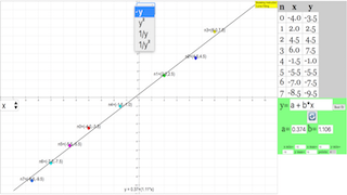
This model fits a polynomial curve to a data set. Users can add points (up to a limit)  by clicking within the plotting panel. Add data to the panel and then adjust the parameters of the polynomial y = f(x), in order to obtain a good fit using the a,b,c,d, and e parameters. Use the best fit button to compare your fit to the the best possible polynomial fit.

NumericJS model element

This model demonstrates how to use theNumeric JSmodel element (see theElementspanel of the model) to solve the system of linear equations required for the least squares approximation.

Reference:Least Squaresentry of theWikipedia.

 

For Teachers Curve Data Fitting

The objective of this model is to fit a curve to a number of points. You can add points (up to a limit)  by clicking on the panel.

Your task is to adjust the parameters of the curve y = f(x), (or the functionf(x)itself!) in order to obtain the best possible fit. You have up to 5 parameters,a,b,c,d, and e.

Edit the "computeBestFit()" method in theCustompanel of the model to edit your best fit algorithm. Then, click on the "Best Fit" button, each time it is displayed in red, to invoke this method.

NumericJS model element

This model uses theNumeric JSmodel element (see theElementspanel of the model) to help you solve the system of linear equations required for the least squares approximation.

Reference: Least Squares entry of the Wikipedia.

Our function is

where{f_j(x)}are a basis of linear independent functions:{1,x,x²,x³,...,x^m}and{c_j}are the coefficients.

The objective is to minimize the sum:

.

To this end, we have to differentiate with respect toc_i, and equate to zero:

Obtaining the follow system:

where (a,b)_dare defined as:

.

Research

[text]

Video

[text]

 Version:

1. http://weelookang.blogspot.sg/2016/06/data-fitting-javascript-html5-applet.html
2. http://www.opensourcephysics.org/items/detail.cfm?ID=13350 original simulation by Francisco Esquembre and Miguel Marín López
   

Other Resources

[text]

FAQ on the Modeling Instruction Data Fitting Applet

1. What is the main purpose of the Data Fitting applet? The primary goal of this applet is to enable users to fit a polynomial curve to a set of data points. Users can add data points by clicking on the plotting panel and then manipulate the curve by adjusting the parameters a, b, c, d, and e of the polynomial function y = f(x) to achieve the best possible fit. This allows exploration of how mathematical models can approximate real-world data.
2. How can I add data points to the applet? You can add data points by simply clicking anywhere within the plotting panel. Note that there may be a limit to the number of data points you can add. These points will then be used as a basis for the curve-fitting process.
3. What is meant by "best fit" in this context? "Best fit" refers to the polynomial curve that most closely approximates the data points. The applet uses the method of least squares approximation (implemented with the Numeric JS model element) to mathematically determine this best-fit curve. The applet also provides a button to invoke a custom “best fit” algorithm.
4. How do I adjust the polynomial curve to fit the data? You adjust the curve by changing the parameters a, b, c, d, and e. These parameters are the coefficients of the polynomial equation y = f(x). By manually changing these coefficients, users can manipulate the shape and position of the curve to closely match the pattern of the data points. The applet offers a numerical input system for precise manipulation of these values.
5. What is the 'NumericJS' model element, and what is its role in this applet? The NumericJS model element is a tool integrated into the applet that performs the mathematical calculations needed for the least squares approximation. This element solves the system of linear equations, which is necessary to determine the best-fit parameters for the polynomial curve. In essence, it automates the process of finding the curve that minimizes the sum of the squared distances between the curve and each data point.
6. What are the linear independent functions in the equation, and why is minimizing the sum important? The functions {1,x,x2,x3,...xm} form a basis of linear independent functions. In this context, they form the building blocks for our polynomial function. The applet's goal is to find the coefficients for these functions that minimize the sum of the squared differences between the predicted y-values (from the polynomial) and the actual y-values of the data points. Minimizing the squared distances ensures that the resulting curve will be as close as possible to all the data points.
7. Where can teachers find the "computeBestFit()" method and how can they modify it? Teachers can access the "computeBestFit()" method in the Custom Panel of the model. They are free to edit the algorithm there, and this custom algorithm will be used when clicking the "Best Fit" button. This feature allows educators to tailor the fitting process and introduce more complex methods beyond the standard least squares approximation.
8. Where can I find more information or the original sources of this model? This model is part of a broader initiative of Open Educational Resources, you can find more information here:
9. http://weelookang.blogspot.sg/2016/06/data-fitting-javascript-html5-applet.html
10. http://www.opensourcephysics.org/items/detail.cfm?ID=13350 (original simulation by Francisco Esquembre and Miguel Marín López) These links will provide context and potentially more details about the creation and use of this interactive simulation.