About

y = f(x) in linear and logarithmic
coordinate systems

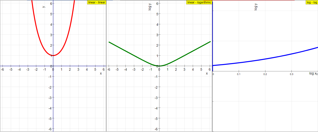
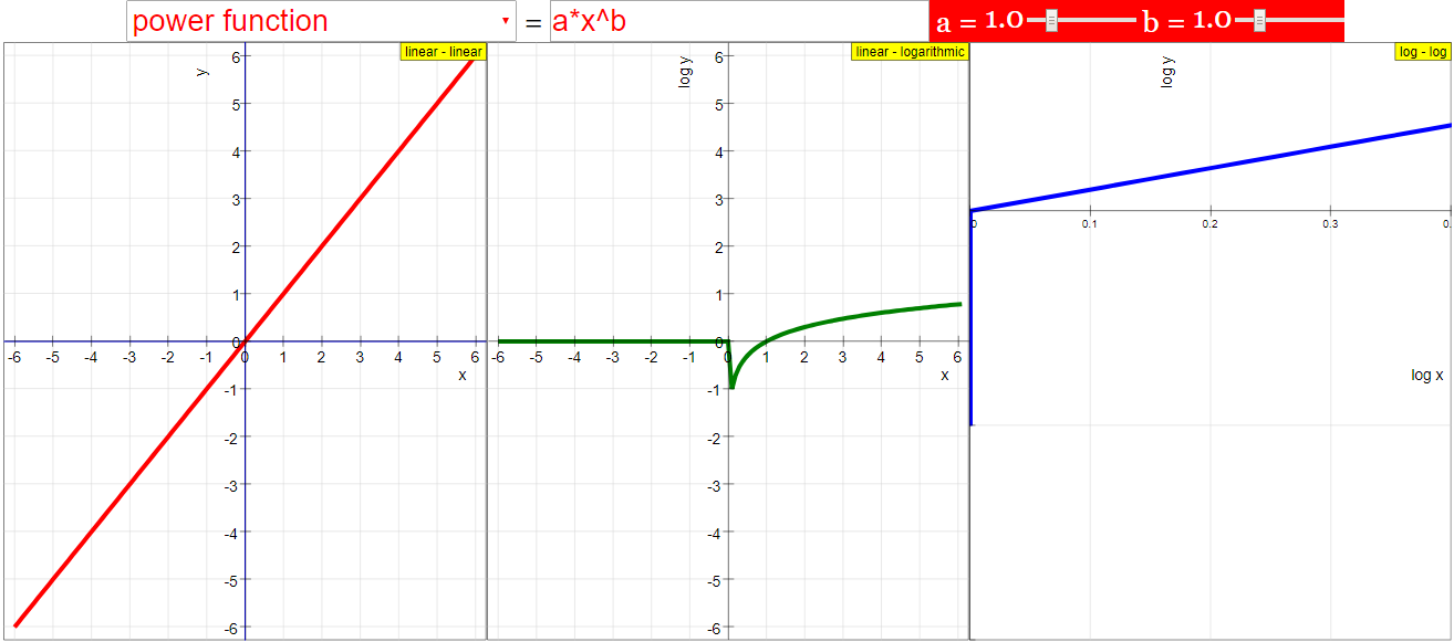
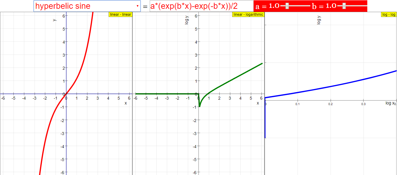
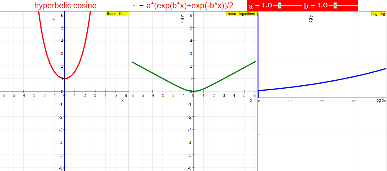
In a coordinate system with linear abscissa scaling and logarithmic ordinate scaling exponential functions appear as straight lines whose gradient is independent of a multiplicative factor.

Potency functions appear as straight lines in a twofold logarithmic coordinate system, with a slope, that indicates the grade of power. Twofold logarithmic coordinate systems emphasize the characteristics at small values of the abscissa by graphical spreading.

Log−linear graphs can only show positive values of the ordinate. Twofold logarithmic graphs are limited to positive values both of ordinate and abscissa. For some of the predefined functions an additive constant avoids cutoffs of negative ordinate values.

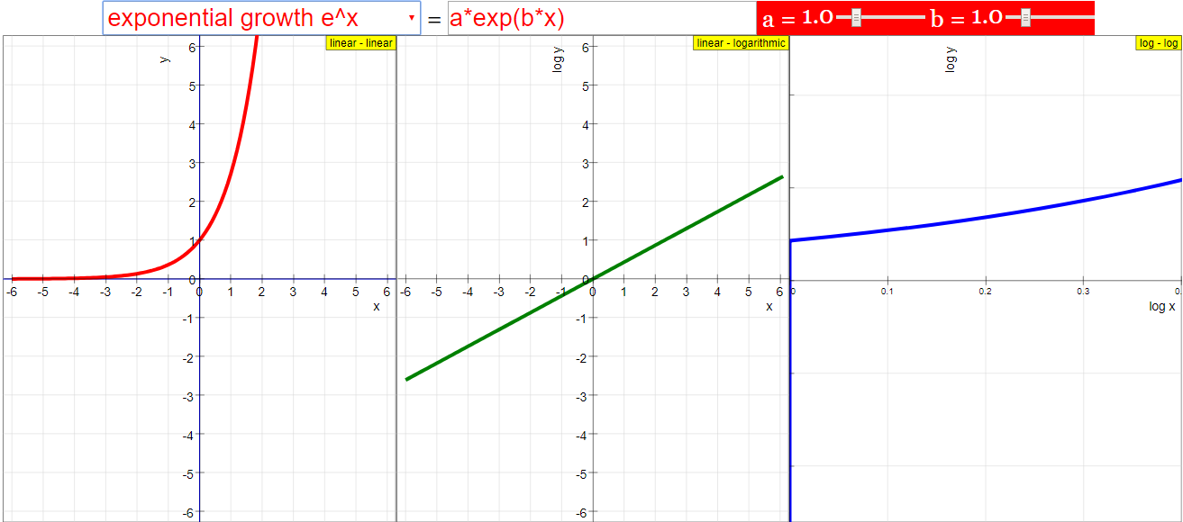
In the default setting three windows of different coordinate scaling show an exponential growth function with two free parameters a = 1 and b = 1. a and b can be varied by sliders. In the linear−linear scheme y = 1 is shown as a red line, and the two coordinate axes are shown as blue lines. The exact value of b appears in an editable number field, in which b is not limited to the range of the slider. Do not forget ENTER after a manual change!

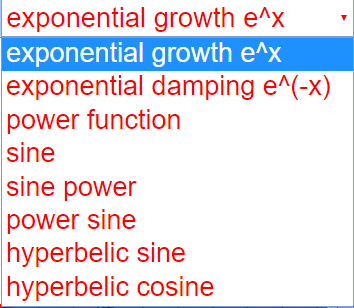
The ComboBox allows selection of a predefined function, whose formula appears in the editable formula field. There you also can input any other function with up to two parameters a and b.

Power functions whose power grade is not an integer will result in imaginary values for negative x values. Only the branch for real x values can be shown. Integers are not easily defined with the slider. Instead, use the number field b to define integer power grades (as 2, 5, 25...)

E 1:  In the default setting compare the three schemes for the exponential growth function. Derive the reason for the visual appearances from the formula.

E 2:  Change parameters a and b and observe the changes of the curves.. What happens at x = 0? Reflect the observation as result of the formula.

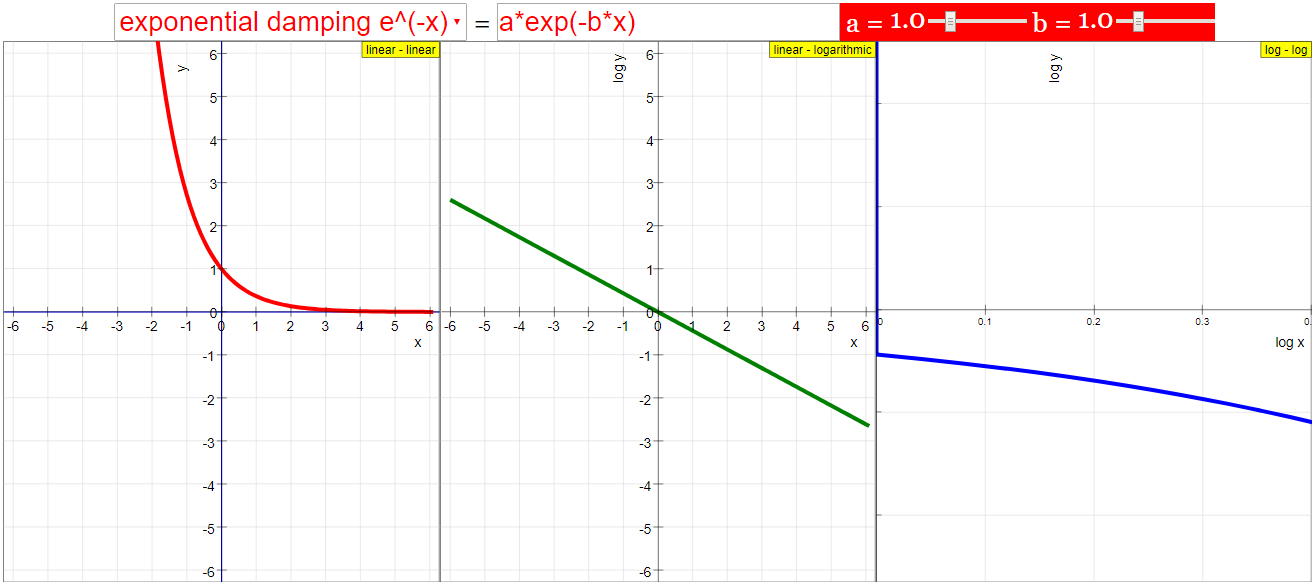
E 3:  Repeat the experiments for exponential damping.

E 4:  Choose the power function. Vary b and study the result in the twofold logarithmic scheme. Compare with the formula.

E 5:  If you choose b with the slider, you probably see just the positive branch in the linear−linear scheme of the potency. Why? Input positive and negative integers into the b text field and study which branches are now shown. Do not hesitate to also choose really high values for b.

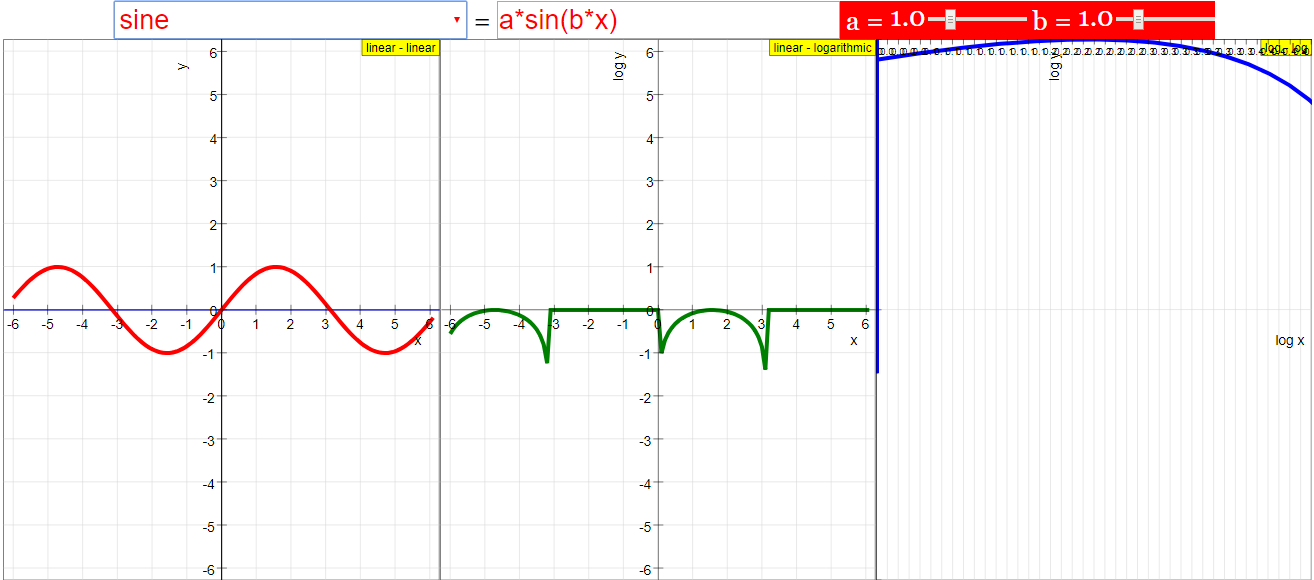
E 6:  Study the appearance of the different periodic functions.

E 7:  Input your own formulas. Use proper factors to stay within the coordinate limits.

E 8: Try to formulate polynomials with several roots in the coordinate range. For some choose even, for others uneven maximum power.

 

Translations

Code	Language		Translator	Run

Credits

Dieter Roess - WEH- Foundation; Fremont Teng; Loo Kang Wee

Overview:

This document reviews a JavaScript simulation applet designed to visualize the behavior of mathematical functions (specifically y = f(x)) when plotted on different coordinate systems: linear-linear, log-linear, and twofold logarithmic. The applet, developed by Open Educational Resources / Open Source Physics @ Singapore, aims to enhance the learning and teaching of mathematics by allowing users to interactively explore how the choice of coordinate system affects the graphical representation of functions, particularly exponential and power functions.

Main Themes and Important Ideas:

1. Impact of Coordinate System Scaling: The core theme is demonstrating how different scaling on the abscissa (x-axis) and ordinate (y-axis) can reveal different properties of functions.

• Linear-linear: This is the standard Cartesian coordinate system where both axes have linear scales.
• Log-linear (linear abscissa, logarithmic ordinate): In this system, exponential functions appear as straight lines. The source explicitly states: "In a coordinate system with linear abscissa scaling and logarithmic ordinate scaling exponential functions appear as straight lines whose gradient is independent of a multiplicative factor." This highlights a key advantage for analyzing exponential growth or decay.
• Twofold logarithmic (logarithmic abscissa and ordinate): Here, power functions are represented as straight lines. The description notes: "Potency functions appear as straight lines in a twofold logarithmic coordinate system, with a slope, that indicates the grade of power." This is valuable for identifying and analyzing power law relationships. Additionally, the source mentions that "Twofold logarithmic coordinate systems emphasize the characteristics at small values of the abscissa by graphical spreading."

1. Interactive Exploration of Functions: The applet allows users to interactively manipulate function parameters and observe the resulting changes in their graphical representations across the three coordinate systems.

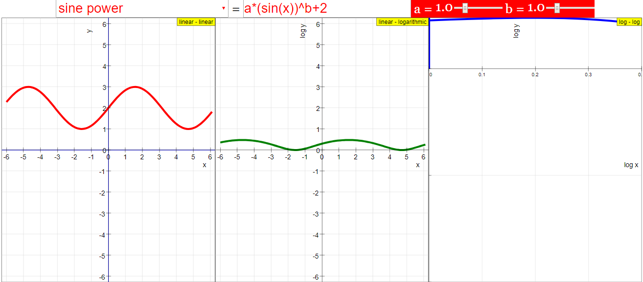
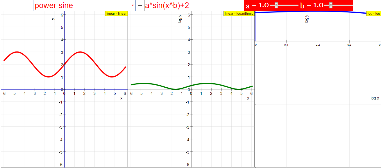
• Users can select predefined functions from a ComboBox, including exponential growth (e^x), exponential damping (e^-x), power functions, sine, sine power, power sine, hyperbolic sine, and hyperbolic cosine.
• The formula of the selected function appears in an editable field, enabling users to input their own functions with up to two parameters, a and b.
• Sliders are provided to vary the parameters a and b for the displayed function. Notably, for parameter b, an editable number field is also available, allowing for more precise input beyond the slider's range, including integer power grades for power functions. The source emphasizes, "Do not forget ENTER after a manual change!"
• The applet displays the chosen function simultaneously in three windows, each with a different coordinate scaling, facilitating direct comparison.

1. Limitations of Logarithmic Scales: The document explicitly points out the limitations of logarithmic coordinate systems:

• "Log−linear graphs can only show positive values of the ordinate."
• "Twofold logarithmic graphs are limited to positive values both of ordinate and abscissa."
• To address the issue of negative ordinate values for some predefined functions, "an additive constant avoids cutoffs of negative ordinate values." This is an important consideration when interpreting graphs on these systems.

1. Experiments for Guided Learning: The "Experiments" section provides a structured approach for users to explore the applet's functionalities and understand the underlying mathematical concepts. These experiments encourage users to:

• Compare the visual appearances of exponential growth and damping across the three schemes and relate them to the function's formula (E1, E3).
• Investigate the effect of changing parameters a and b on the curves and analyze the behavior at x = 0 (E2).
• Study power functions in the twofold logarithmic scheme and compare the results with the formula, particularly focusing on how the exponent b influences the slope (E4, E5).
• Examine the appearance of periodic functions (E6).
• Input their own formulas and polynomials (E7, E8).

1. Educational Resource: The applet is presented as an open educational resource for learning and teaching mathematics, particularly within the context of physics examples. Its inclusion in the "Learning and Teaching Mathematics using Simulations – Plus 2000 Examples from Physics" category underscores this purpose. The availability of an Embed code allows educators to integrate the simulation directly into web pages.
2. Technical Details: The applet is a JavaScript simulation (HTML5), making it accessible through web browsers without the need for additional plugins. The credits acknowledge the developers, Dieter Roess, Fremont Teng, and Loo Kang Wee.

Key Quotes:

• "In a coordinate system with linear abscissa scaling and logarithmic ordinate scaling exponential functions appear as straight lines whose gradient is independent of a multiplicative factor."
• "Potency functions appear as straight lines in a twofold logarithmic coordinate system, with a slope, that indicates the grade of power."
• "Twofold logarithmic coordinate systems emphasize the characteristics at small values of the abscissa by graphical spreading."
• "Log−linear graphs can only show positive values of the ordinate."
• "Twofold logarithmic graphs are limited to positive values both of ordinate and abscissa."
• "Do not forget ENTER after a manual change!"

Conclusion:

The "Function in Linear and Logarithmic Coordinate Systems JavaScript Simulation Applet HTML5" is a valuable interactive tool for understanding the impact of different coordinate system scalings on the graphical representation of functions, especially exponential and power functions. Its user-friendly interface, predefined functions, parameter manipulation capabilities, and guided experiments make it an effective resource for both students and educators in mathematics and related fields. The explicit mention of the limitations of logarithmic scales ensures a comprehensive understanding of their appropriate use. The applet's availability as an open educational resource further enhances its accessibility and potential for widespread adoption in learning environments.

Study Guide: Linear and Logarithmic Coordinate Systems

Key Concepts

• Linear Coordinate System: A standard Cartesian coordinate system where both the x-axis (abscissa) and y-axis (ordinate) have linear scales. Equal distances on the axes represent equal changes in value.
• Log-Linear Coordinate System: A coordinate system with a linear scale on the x-axis (abscissa) and a logarithmic scale on the y-axis (ordinate). This is useful for visualizing exponential relationships as straight lines.
• Twofold Logarithmic Coordinate System (Log-Log): A coordinate system where both the x-axis (abscissa) and y-axis (ordinate) have logarithmic scales. This is useful for visualizing power law relationships as straight lines.
• Exponential Function (y = a * b^x): A function where the independent variable (x) appears in the exponent. In a log-linear plot, this function appears as a straight line. The gradient of the line is related to the base 'b', and the y-intercept is related to the coefficient 'a'.
• Power Function (y = a * x^b): A function where the independent variable (x) is raised to a power (b). In a twofold logarithmic plot, this function appears as a straight line. The slope of the line is equal to the exponent 'b', and the y-intercept is related to the coefficient 'a'.
• Gradient/Slope: The rate of change of a function, represented visually by the steepness of a line on a graph. In log-linear plots of exponential functions, the gradient is independent of a multiplicative factor. In log-log plots of power functions, the slope indicates the grade of power.
• Multiplicative Factor: A constant that multiplies a variable or function.
• Additive Constant: A constant that is added to a variable or function. In the context of the simulation, an additive constant can be used to shift a function vertically and avoid cutoffs of negative ordinate values in logarithmic plots.
• Parameters (a and b): Adjustable constants in a function that determine its specific form and behavior. In the simulation, sliders and editable number fields allow for the manipulation of these parameters.
• Predefined Functions: Common mathematical functions (e.g., exponential growth, exponential damping, power function, sine, cosine) that are available for selection in the simulation.
• Formula Field: An editable text box in the simulation where users can view and input mathematical functions, including those with parameters 'a' and 'b'.
• Sliders: Interactive graphical elements in the simulation that allow users to continuously vary the values of parameters, typically within a defined range.
• Number Field: An editable text box in the simulation where users can directly input numerical values for parameters, potentially outside the range of the associated slider.

Quiz

1. In what type of coordinate system does an exponential function appear as a straight line? What property of the line is related to the base of the exponential function?
2. Explain why a twofold logarithmic coordinate system is particularly useful for visualizing potency (power) functions. What does the slope of the line in such a plot represent?
3. What are the limitations regarding the values of the ordinate (y-axis) that can be displayed on a log-linear graph? What about a twofold logarithmic graph? Why do these limitations exist?
4. Describe the visual representation of the function y = 1 in the linear-linear scheme of the simulation's default setting. What do the blue lines represent in this scheme?
5. How can you change the parameters 'a' and 'b' of a function within the simulation applet? What is a key difference in how the 'b' parameter can be adjusted?
6. What happens when you input a power function with a non-integer power grade and negative x values? Why does the simulation typically only show the positive branch in the linear-linear scheme when using the slider for the power grade?
7. Where in the simulation can you select from predefined functions and also input your own formulas? How many parameters can a user-defined function have in this simulation?
8. What does Experiment E1 suggest you do? What are you expected to deduce by performing this experiment?
9. According to the text, what should you remember to do after manually changing a value in the editable number field for parameter 'b'? Why is this step important?
10. What does the "Function Box" toggle in the simulation? What information does it provide for each panel?

Answer Key

1. An exponential function appears as a straight line in a log-linear coordinate system (linear abscissa, logarithmic ordinate). The gradient (slope) of this straight line is independent of a multiplicative factor and is related to the base 'b' of the exponential function.
2. A twofold logarithmic coordinate system is useful for visualizing power functions because they appear as straight lines in such a plot. The slope of the line in a twofold logarithmic plot of a power function indicates the grade of the power (the exponent 'b').
3. Log-linear graphs can only show positive values of the ordinate because the logarithm of a non-positive number is undefined. Twofold logarithmic graphs are limited to positive values for both the ordinate and abscissa for the same reason.
4. In the linear-linear scheme, y = 1 is shown as a red horizontal line. The two coordinate axes (x-axis and y-axis) are shown as blue lines.
5. The parameters 'a' and 'b' can be changed using sliders in the control panel or by directly editing the values in the editable number field. A key difference is that the slider for 'b' has a limited range, while the number field allows for inputting values outside that range, including integers which are not easily defined with the slider.
6. Power functions with a non-integer power grade will result in imaginary values for negative x values, so only the branch for real x values can be shown. The slider for 'b' likely has a range that primarily explores positive values, leading to the observation of just the positive branch in the linear-linear scheme for potency functions.
7. You can select from predefined functions and input your own formulas in the editable formula field, which appears after selecting a predefined function or by directly typing. User-defined functions in this simulation can have up to two parameters, 'a' and 'b'.
8. Experiment E1 suggests comparing the three coordinate schemes (linear-linear, log-linear, twofold logarithmic) for the exponential growth function in the default setting. You are expected to derive the reason for the different visual appearances of the curve in each scheme based on the mathematical formula of the exponential function and the nature of the coordinate scaling.
9. After manually changing a value in the editable number field for parameter 'b', you must press the "ENTER" key for the change to be registered and reflected in the simulation. This step is important because the simulation only updates the parameter value when the "ENTER" key is pressed after manual input.
10. The "Function Box" toggles the display of the respective functions and their resulting graphs in each of the coordinate system panels. It shows the mathematical formula of the selected function.

Essay Format Questions

1. Discuss the advantages and limitations of using log-linear and twofold logarithmic coordinate systems compared to linear-linear systems when analyzing different types of mathematical functions. Provide specific examples of functions and explain how the logarithmic scales facilitate their interpretation.
2. Explain the relationship between the parameters 'a' and 'b' in exponential functions and their graphical representation in linear-linear and log-linear coordinate systems, as explored through the simulation's controls and Experiment E2. How do changes in these parameters affect the appearance of the graph in each system?
3. Consider the behavior of power functions with different integer and non-integer exponents, particularly when dealing with negative values of the abscissa. Explain why the twofold logarithmic plot is useful for analyzing the positive branches of these functions, as suggested by Experiment E4 and E5.
4. Describe how the JavaScript simulation applet allows users to explore the relationship between mathematical formulas and their graphical representations in different coordinate systems. Discuss the interactive features, such as the ComboBox, formula field, and sliders, and how they contribute to a deeper understanding of function behavior.
5. Based on the experiments suggested (E1-E8), outline a series of investigations a student could conduct using the simulation to understand the visual characteristics of exponential, power, and periodic functions in linear, log-linear, and twofold logarithmic coordinate systems. What key insights should the student gain from these investigations?

Glossary of Key Terms

• Abscissa: The horizontal coordinate (x-coordinate) in a two-dimensional Cartesian coordinate system.
• Ordinate: The vertical coordinate (y-coordinate) in a two-dimensional Cartesian coordinate system.
• Linear Scaling: A scale where equal intervals represent equal numerical differences.
• Logarithmic Scaling: A scale where equal intervals represent equal ratios or multiplicative factors.
• Exponential Growth: A type of function where the value increases rapidly over time, proportional to its current value (typically of the form y = a * b^x where b > 1).
• Exponential Damping: A type of function where the value decreases rapidly over time (typically of the form y = a * b^x where 0 < b < 1 or y = a * e^(-kx) where k > 0).
• Potency Function: Another term for a power function, where one variable is raised to a constant power.
• Gradient: The slope of a line, representing the rate of change.
• Parameter: A variable that is held constant for a particular instance but can vary between instances or contexts (e.g., 'a' and 'b' in y = a * x^b).
• Simulation Applet: A small application, often web-based and interactive, that models a real-world system or mathematical concept.
• ComboBox: A drop-down list or menu allowing users to select from a predefined set of options.

Sample Learning Goals

[text]

For Teachers

Function in Linear and Logarithmic Coordinate Systems JavaScript Simulation Applet HTML5

Instructions

Function Box

Editing the Functions

Toggling Full Screen

Research

[text]

Video

[text]

 Version:

Other Resources

[text]

Frequently Asked Questions about Linear and Logarithmic Coordinate Systems Simulation

1. What is the purpose of the "Function in Linear and Logarithmic Coordinate Systems" JavaScript simulation?

This simulation allows users to visualize the graph of a function, y = f(x), across three different coordinate systems: linear-linear, linear-logarithmic, and twofold logarithmic. This helps in understanding how different coordinate scalings affect the visual representation of various types of functions, such as exponential and power functions.

2. How do exponential functions appear in different coordinate systems within the simulation?

In a coordinate system with a linear x-axis and a logarithmic y-axis (log-linear), exponential functions appear as straight lines. The slope of this line is related to the rate of exponential growth or decay and is independent of any multiplicative factor in the function. In a linear-linear system, exponential functions are curves, while in a twofold logarithmic system, they will also appear as curves.

3. What is unique about how power functions are displayed in a twofold logarithmic coordinate system?

In a twofold logarithmic coordinate system (where both the x and y axes have logarithmic scaling), power functions appear as straight lines. The slope of this straight line directly corresponds to the exponent (or "grade of power") of the power function. This representation makes it easier to determine the power relationship between the variables.

4. What are the limitations of using log-linear and twofold logarithmic graphs as highlighted by the simulation?

Log-linear graphs are restricted to displaying only positive values on the y-axis (ordinate). Twofold logarithmic graphs have a stricter limitation, as they can only display positive values for both the x-axis (abscissa) and the y-axis. The simulation sometimes uses an additive constant for predefined functions to avoid cutoffs of negative y-values in log-linear views.

5. How can users interact with the simulation to explore different functions?

Users can interact with the simulation in several ways:

• ComboBox: Select from a list of predefined functions (e.g., exponential growth, exponential damping, power function, trigonometric functions).
• Editable Formula Field: Input their own function formulas with up to two parameters, a and b.
• Sliders: Adjust the values of the parameters a and b for the displayed function (note that the range of the slider might be limited).
• Editable Number Field: For the parameter b, there is an editable number field where users can input values outside the slider's range, including integers for power functions. Remember to press "ENTER" after manual changes.

6. What experiments are suggested within the simulation to aid learning?

The simulation suggests several experiments, including:

• Comparing the visual appearance of exponential growth and damping functions across the three coordinate systems and relating it to their formulas.
• Observing how changing the parameters a and b affects the curves in each coordinate system, particularly noting behavior at x = 0.
• Studying the representation of power functions in the twofold logarithmic scheme and comparing it to the formula, including investigating the display of positive and negative branches based on integer powers.
• Examining the appearance of periodic functions.
• Inputting custom formulas and polynomials to see their graphical representations in different coordinate systems.

7. Why might only a positive branch of a power function be visible in the linear-linear scheme when using the slider for the exponent?

When using the slider to define the exponent of a power function, you might primarily see the positive branch in the linear-linear scheme because non-integer powers of negative numbers result in imaginary values, which cannot be displayed on a standard real-valued Cartesian plane. By inputting positive and negative integers in the dedicated number field for the exponent b, you can observe how different branches of the power function are displayed for real x values.

8. Where can this simulation be embedded and what are the licensing terms for its use?

The simulation can be embedded in a webpage using the provided iframe code. The content of the Open Educational Resources / Open Source Physics @ Singapore website, including this simulation, is licensed under the Creative Commons Attribution-Share Alike 4.0 Singapore License. For commercial use of the underlying EasyJavaScriptSimulations Library, separate licensing terms apply, and users should contact fem@um.es directly for details.