
.png
)


About
Developed by W. Freeman
The standard description of the behavior of the vibrating string is only valid in the low-amplitude limit. In this exercise, students build a lattice-elasticity model of a vibrating string and then study its properties, first verifying that the standard properties predicted by hold in the low-amplitude limit and then studying the nonlinear properties of the vibrating string as the amplitude increases.
| Subject Areas | Waves & Optics, Mathematical/Numerical Methods, and Other |
|---|---|
| Levels | Beyond the First Year and Advanced |
| Available Implementation | C/C++ |
| Learning Objectives |
|
| Time to Complete | 90-360 min |
#include <stdio.h>
#include <stdlib.h>
#include <math.h>
#include <time.h>
// #define ONE_PERIOD_ONLY // uncomment this to do only one period, then print stats and exit.
void get_forces(double *x, double *y, double *Fx, double *Fy, int N, double k, double r0) // pointers here are array parameters
{
int i;
double r;
Fx[0]=Fy[0]=Fx[N]=Fy[N]=0; // have to set the end forces properly to avoid possible uninitialized memory shenanigans
double U=0,E=0,T=0;
for (i=1;i<N;i++)
{
// left force
r = hypot(x[i]-x[i-1],y[i]-y[i-1]);
Fx[i] = -(x[i]-x[i-1]) * k * (r-r0)/r;
Fy[i] = -(y[i]-y[i-1]) * k * (r-r0)/r;
// right force
r = hypot(x[i]-x[i+1],y[i]-y[i+1]);
Fx[i] += -(x[i]-x[i+1]) * k * (r-r0)/r;
Fy[i] += -(y[i]-y[i+1]) * k * (r-r0)/r;
}
}
void evolve_euler(double *x, double *y, double *vx, double *vy, int N, double k, double m, double r0, double dt)
{
int i;
double Fx[N+1],Fy[N+1]; // this could be made faster by mallocing this once, but we leave it this way for students
// to avoid having to deal with malloc(). In any case memory allocation is faster than a bunch
// of square root calls in hypot().
get_forces(x,y,Fx,Fy,N,k,r0);
for (i=1;i<N;i++)
{
x[i] += vx[i]*dt;
y[i] += vy[i]*dt;
vx[i] += Fx[i]/m*dt;
vy[i] += Fy[i]/m*dt;
}
}
// this function is around to go from Euler-Cromer to leapfrog, if we want second-order precision
void evolve_velocity_half(double *x, double *y, double *vx, double *vy, int N, double k, double m, double r0, double dt)
{
int i;
double Fx[N+1],Fy[N+1]; // this could be made faster by mallocing this once, but we leave it this way for students
get_forces(x,y,Fx,Fy,N,k,r0);
for (i=1;i<N;i++)
{
vx[i] += Fx[i]/m*dt/2;
vy[i] += Fy[i]/m*dt/2;
}
}
// Students might not be familiar with pass-by-reference as a trick for returning multiple values yet.
// Ideally they should be coding this anyway, and there are a number of workarounds, in particular
// just not using a function for this.
void get_energy(double *x, double *y, double *vx, double *vy, int N, double k, double m, double r0, double *E, double *T, double *U)
{
*E=*T=*U=0;
int i;
double r;
for (i=0;i<N;i++)
{
*T+=0.5*m*(vx[i]*vx[i] + vy[i]*vy[i]);
r = hypot(x[i]-x[i+1],y[i]-y[i+1]);
*U+=0.5*k*(r-r0)*(r-r0);
}
*E=*T+*U;
}
// does what it says on the tin
void evolve_euler_cromer(double *x, double *y, double *vx, double *vy, int N, double k, double m, double r0, double dt)
{
int i;
double Fx[N+1],Fy[N+1]; // this could be made faster by mallocing this once, but we leave it this way for students
for (i=1;i<N;i++)
{
x[i] += vx[i]*dt;
y[i] += vy[i]*dt;
}
get_forces(x,y,Fx,Fy,N,k,r0);
for (i=1;i<N;i++)
{
vx[i] += Fx[i]/m*dt;
vy[i] += Fy[i]/m*dt;
}
}
// does what it says on the tin
void evolve_rk2(double *x, double *y, double *vx, double *vy, int N, double k, double m, double r0, double dt)
{
int i;
double Fx[N+1],Fy[N+1]; // this could be made faster by mallocing this once, but we leave it this way for students
double xh[N+1],yh[N+1],vxh[N+1],vyh[N+1];
vxh[0]=vyh[0]=vxh[N]=vyh[N]=0;
get_forces(x,y,Fx,Fy,N,k,r0);
for (i=0;i<=N;i++)
{
xh[i] = x[i] + vx[i]*dt/2;
yh[i] = y[i] + vy[i]*dt/2;
vxh[i] = vx[i] + Fx[i]/m*dt/2;
vyh[i] = vy[i] + Fy[i]/m*dt/2;
}
get_forces(xh,yh,Fx,Fy,N,k,r0);
for (i=0;i<=N;i++) // need two for loops -- can't interleave halfstep/fullstep updates (students have trouble with this sometimes!)
{
x[i] = x[i] + vx[i]*dt;
y[i] = y[i] + vy[i]*dt;
vx[i] = vx[i] + Fx[i]/m*dt;
vy[i] = vy[i] + Fy[i]/m*dt;
}
}
// function to encapsulate determining whether we need to shovel another frame to the animator. delay is the delay in msec.
// I usually aim to hide library calls, like clock() and CLOCKS_PER_SEC, from students in the beginning, since it's not really
// relevant to their development of computational skills, which are what I really care about.
int istime(int delay)
{
static int nextdraw=0;
if (clock() > nextdraw)
{
nextdraw = clock() + delay * CLOCKS_PER_SEC/1000.0;
return 1;
}
return 0;
}
int main(int argc, char **argv)
{
int i,N=80; // number of links, not number of nodes!! Careful for the lurking fencepost errors
int modenumber=3; // put in some defaults just in case
double t, dt=2e-6, amplitude=0.1;
double stiffness=10, density=1, length=1; // unstretched properties of original string
double k, m, r0; // properties of single string
double tension=1,Ls;
if (argc < 9) // if they've not given me the parameters I need, don't just segfault -- tell the user what to do, then let them try again
{
printf("!Usage: <this> <N> <modenumber> <dt> <amplitude> <stiffness> <density> <length> <tension>\n");
exit(0);
}
N=atoi(argv[1]);
modenumber=atoi(argv[2]);
dt=atof(argv[3]);
amplitude=atof(argv[4]);
stiffness=atof(argv[5]);
density=atof(argv[6]);
length=atof(argv[7]);
tension=atof(argv[8]);
double x[N+1], y[N+1], vx[N+1], vy[N+1], E, T, U;
// compute microscopic properties from macroscopic ones
r0=length/N;
m=density*length/N;
k=stiffness*N/length;
// figure out stretched length
Ls=length + tension * length / stiffness;
// make predictions based on what our freshman mechanics class taught us
double density_stretched = density * length / Ls;
double wavespeed = sqrt(tension/density_stretched);
double period_predict = 2 * Ls / wavespeed / modenumber;
double vym_last=0;
int monitor_node = N/modenumber/2; // this is the node that we'll be watching to see when a period has elapsed.
int nperiods=0;
for (i=0;i<=N;i++) // remember, we have N+1 of these
{
x[i] = Ls*i/N;
y[i] = amplitude*sin(modenumber * M_PI * x[i] / Ls);
vx[i]=0;
vy[i]=0;
}
// now, loop over time forever...
printf("!N\tmode\tgamma\t\tL\t\tamp.\t\tdens.\tTension\tT\tT_pred\tDelta\t\tFreq (Hz)\n"); // print header
for (t=0;1;t+=dt)
{
vym_last=vy[monitor_node];
evolve_euler_cromer(x,y,vx,vy,N,k,m,r0,dt);
// "if we were going up, but now we're going down, then a period is complete"
// this is crude and will fail if it has enough "wobble", but it's sufficient for this project.
if (vym_last > 0 && vy[monitor_node] < 0)
{
nperiods++;
printf("!%d\t%d\t%.2e\t%.2e\t%.4e\t%.1e\t%.1e\t%.4f\t%.4f\t%.4e\t%.4e\n",N,
modenumber,stiffness,length,amplitude,density,tension,t,period_predict*nperiods,1-t/period_predict/nperiods,nperiods/t);
#ifdef ONE_PERIOD_ONLY
printf("Q\n"); // kill anim before we die ourselves
exit(1);
#endif
}
if (istime(15)) // wait 15ms between frames sent to anim; this gives us about 60fps.
{
printf("C 1 0 0\nc %f %f 0.02\nC 1 1 1\n",x[monitor_node],y[monitor_node]); // draw a big red blob around the node we're watching
for (i=0;i<=N;i++)
{
printf("C %e 0.5 %e\n",0.5+y[i]/amplitude,0.5-y[i]/amplitude); // use red/blue shading; this will make vibrations visible even if amp<<1
printf("c %f %f %f\n",x[i],y[i],length/N/3); // draw circles, with radius scaled to separation
if (i<N) printf("l %f %f %f %f\n",x[i],y[i],x[i+1],y[i+1]); // the if call ensures we don't drive off the array
}
printf("T -0.5 -0.7\ntime = %f\n",t);
get_energy(x,y,vx,vy,N,k,m,r0,&E,&T,&U);
printf("T -0.5 -0.63\nenergy = %e + %e = %e\n",T,U,E);
printf("F\n"); // flush frame
}
}
}
Part 1: Modeling
The goal of this project is to numerically calculate the vibrations of a stretched string of total mass , unstretched length , Young’s modulus , and cross-sectional area .You will do this by modeling it as a series of point masses of mass connected by Hooke’s-law springs, each of equilibrium length and spring constant .
Recall that the spring constant of the overall spring is given by . The variables and only appear in the combination ; it is useful to define this as the “stiffness”, .
- What mass should the point masses have, and what equilibrium length and spring constant should the springs have, in order for the properties of the model to match the properties of the string itself?
Part 2: Coding
Now you will use a computer program to calculate numerically the behavior of this model of the vibrating string, since it is just a collection of objects (two of which are held fixed, at either end) moving under the influence of calculable forces (from the Hooke’s-law springs).
-
How many dynamical variables will you need to update during each integration step? What are they?
-
Each mass feels forces from the two springs that connect it to the two adjacent masses. Write an expression for the net force on mass in terms of the model parameters and the positions of the other masses. (It may be cleaner if you do this in several steps, defining intermediate variables for the separation magnitudes involved. It may also make your code cleaner to introduce such an intermediate variable; remember, memory is cheap!)
As a reminder: Hooke’s law says that a spring with endpoints at and exerts a force on the endpoint at equal to
where is a vector pointing from A to B.
- Once you understand how to calculate the force on all the masses, write code to numerically integrate Newton’s law of motion for the system. At first, do this with the Euler-Cromer integrator. Some hints:
1) You’ll need to store the dynamical variables in arrays. If you are
using C, remember that arrays are passed to and “returned from”
functions in a different way than single numbers. However, it may be
quite helpful to write functions with names like get_forces() and evolve_euler_cromer().
2) Remember that the Euler-Cromer prescription is to update the
positions based on the velocities, then compute the acceleration from
the new positions and update the velocities. However, you need to update allthe
positions first, then all the
velocities. Otherwise you’ll be in a situation where a given update uses
old data for the left neighbor and new data for the right neighbor, or
vice-versa, and you’ll get results that depend on which way you run your for loop
(which is clearly not right).
3) There is a famous riddle: “A farmer wants to build a
hundred-foot-long fence with fenceposts every ten feet. How many
fenceposts does she need?” The answer is not ten, but eleven; answering
“ten” here is called a “fencepost error” in computing. Note that you have springs
and masses,
but that the first and last of these do not move. This, combined with
the fact that your programming language probably uses zero-indexed
arrays (so an array of 100 things is numbered 0 to 99) means that you
will need to think clearly about the bounds of your for loops.
Part 3: Testing
Once you have your numerical solver coded, you will need to supply initial conditions. At first, consider a stretched but unexcited string, where the two endpoints are held fixed at some distance such that the spring bears a tension .
-
In terms of the string parameters and , and the tension , what is ? (That is, how far must you stretch your string to achieve the desired tension?)
-
In terms of and your number of segments , what initial conditions for the ’s and ’s correspond to this stretched but unexcited string?
-
Code these initial conditions and verify that your string doesn’t move. If you haven’t already, make your program animate your vibrating string using your favorite visualization tool.
-
Now, excite your string by displacing it in some fashion and verify qualitatively that it moves realistically. Note that if you choose the simplest thing and displace only one point mass, this corresponds to “whacking a guitar string with a knife”; you will get rather violent oscillations in this case.
-
Modify your program to track conservation of energy. The kinetic energy is just the sum of for all the masses, and the potential energy is the sum of for all the springs. Verify that your simulation approximately conserves energy.
Part 4: The low-amplitude limit, qualitatively
If the vibrational amplitude is sufficiently small, the trigonometric functions involved in the geometry here can be replaced with the first nontrivial term in their Taylor series. (These are often called the “small-angle approximations.) When this is done, the system becomes perfectly linear and can be shown to obey the classical wave equation. This leads to the behavior you are probably familiar with, characterized by three main properties:
1) The “normal modes”, oscillatory patterns of definite frequency, are sine waves with a node at either end (and possibly other nodes in the middle). Specifically, the th normal mode is given by
2) The frequencies are given by
3) Since the system (in the ideal, low-amplitude case! – which is all you can solve easily without the computer) is perfecty linear, any number of normal modes, with any amplitudes, can coexist on the string without interfering. Any arbitrary excitation – like a plucked guitar string – is a superposition of many different normal modes with different amplitudes.
Let’s now see how well your string model reproduces these ideal properties.
-
Write initial-condition code to excite your string in any given normal mode with any given amplitude. Using a tension sufficient to stretch your string by at least twenty percent of its original length, try different normal modes at various amplitudes (ranging from “barely visible” to “large”). Does your model reproduce the expected qualitative behavior of the ideal vibrating string? In which regimes?
-
How does the behavior depend on the number of masses you have chosen? Should this affect the behavior at all? Is using a large more critical for modeling the low- normal modes, or the high ones? Why?
-
Now, write initial-condition code to excite your string with a Gaussian bump with any given width and location. Excite your string with narrow and wide Gaussians of modest amplitude, located both near the endpoints and near the center of the string. By observing the animation, comment on whether you have excited mostly the lower normal modes, or the higher ones.
-
If you have access to a stringed instrument (guitar, violin, ukelele, etc.), excite your real string in these ways (by plucking it with both your thumb and the edge of your fingernail, both near the center of the string and near the endpoint). How does the timbre of the sound produced correspond to the answers to your previous question?
Part 5: The low-amplitude limit, quantitatively
Now, let’s study the string’s vibrations precisely, and determine how well and under what conditions they align with the analytic predictions.
The quantitative thing that we can measure is the string’s period. To measure the period of any given normal mode , select a mass near an antinode of that mode, and watch it move up and down. If your initial conditions displace the string in the +y direction, then the string has completed one full period when the string moves “down, then back up, then starts to go down again”. To have our program tell us when that is, we want to watch for the time when the velocity changes from positive to negative.
In order to detect this, you’ll need to introduce a variable that keeps track of the previous value of at that position, so you can monitor it for sign changes.
- Modify your code to track the period, and measure the period of a normal mode of your choice. How does your result correspond to the analytic prediction in the low-amplitude regime for different normal modes? Vary the tension, mass, Young’s modulus, and length, and see if your simulation behaves as expected.
Part 6: Getting away from the low-amplitude limit
All of the things you’ve learned about the vibrating string – noninterfering superpositions of normal modes whose frequency is independent of amplitude – relate to solutions of the ideal wave equation. But deriving this equation from our model requires making the small-angle approximation to trigonometric functions, and this is only valid in the limit . Now it’s time to do something the pen-and-paper crowd can’t do (without a great deal of pain): get away from that limit.
- Try running your simulation at higher amplitudes using a variety of initial conditions. Play with this for a while. Do you still see well-defined normal modes with a constant frequency that “stay put”? Look carefully at the motion of each point; do they still move only up and down? Describe your observations.
Translations
| Code | Language | Translator | Run | |
|---|---|---|---|---|
 |
||||
Credits

Fremont Teng; Loo Kang Wee; based on codes by W. Freeman
Overview
This document summarizes the key themes and important ideas presented in the provided excerpts. The source describes a computational exercise where students develop and analyze a lattice-elasticity model of a vibrating string. This model, unlike the standard wave equation which is valid only for small amplitudes, allows for the study of nonlinear properties of the string as the amplitude of vibration increases. The exercise is divided into parts, guiding students through building the model, coding a numerical solver, testing its behavior in the low-amplitude limit against analytical predictions, and finally exploring nonlinear effects at larger amplitudes.
Main Themes and Important Ideas
1. Limitations of the Standard Vibrating String Model:
- The traditional description of a vibrating string using the wave equation is accurate only when the amplitude of vibrations is small. The source explicitly states: "The standard description of the behavior of the vibrating string is only valid in the low-amplitude limit."
- This limitation arises from the "small-angle approximation to trigonometric functions" used in deriving the wave equation from a more fundamental model.
2. Introduction of the Lattice-Elasticity Model:
- To overcome the limitations of the standard model, the exercise introduces a lattice-elasticity model. This model represents the string as a series of discrete point masses connected by Hooke's law springs.
- The goal is to "build a lattice-elasticity model of a vibrating string and then study its properties, first verifying that the standard properties predicted by \(v = \sqrt{T/\mu}\) hold in the low-amplitude limit and then studying the nonlinear properties of the vibrating string as the amplitude increases."
- The model's parameters (masses, spring constants, equilibrium length) are related to the macroscopic properties of the string (total mass \(M\), unstretched length \(L\), Young’s modulus \(Y\), and cross-sectional area \(A\)). The "stiffness" \(\gamma \equiv AY\) is defined as a useful parameter.
3. Numerical Calculation of Vibrations:
- A key aspect of the project is the numerical calculation of the string's vibrations using the lattice model. Since the model consists of discrete objects moving under calculable forces, its behavior can be simulated computationally.
- The force between adjacent masses is governed by Hooke's law: "\(\vec{F}{BA} = k (r{AB} - r_0) \hat{r}{AB}\)", where \(k\) is the spring constant, \(r{AB}\) is the distance between masses A and B, and \(r_0\) is the equilibrium length.
- The project requires students to code a numerical solver to simulate the motion of these masses over time.
4. Testing and Verification in the Low-Amplitude Limit:
- The exercise emphasizes the importance of testing the numerical model by comparing its predictions to the analytical results known for the standard vibrating string in the low-amplitude regime.
- Students are instructed to supply initial conditions corresponding to a stretched but unexcited string and then to introduce excitations corresponding to normal modes.
- The analytical solution for the \(n\)-th normal mode is given as "\(y(x, t) = A \sin \frac{n \pi x}{L'} \cos \omega_n t\)", where \(L'\) is the stretched length and \(\omega_n\) is the angular frequency. The relationship between frequency, wavespeed, and wavelength is also mentioned: "\(f_n = \omega_n / 2\pi = n v / 2L'\)".
- The wavespeed \(v\) in this limit is given by "\(v = \sqrt{T / \mu'}\)", where \(T\) is the tension and \(\mu'\) is the linear mass density of the stretched string.
5. Quantitative Measurement of Period:
- To quantitatively compare the simulation with analytical predictions in the low-amplitude limit, students are tasked with measuring the period of the normal modes in their simulation.
- The suggested method involves tracking the vertical velocity of a mass near an antinode and detecting when it completes a full cycle.
- Students are asked to "modify your code to track the period, and measure the period of a normal mode of your choice. How does your result correspond to the analytic prediction in the low-amplitude regime for different normal modes? Vary the tension, mass, Young’s modulus, and length, and see if your simulation behaves as expected."
6. Exploring Nonlinearity at Large Amplitudes:
- The ultimate goal of using the lattice model is to investigate the behavior of the vibrating string beyond the low-amplitude limit, where nonlinear effects become significant.
- The source highlights that the standard wave equation relies on approximations that break down at larger amplitudes: "deriving this equation from our model requires making the small-angle approximation to trigonometric functions, and this is only valid in the limit \(A \rightarrow 0\)."
- The exercise encourages students to explore phenomena that are not captured by the ideal wave equation, emphasizing the power of numerical simulation: "Now it’s time to do something the pen-and-paper crowd can’t do (without a great deal of pain): get away from that limit."
7. Dependence on the Number of Masses (N):
- The source prompts students to consider the impact of the discretization (number of masses \(N\)) on the simulation's behavior.
- Questions are raised about whether \(N\) should affect the behavior and whether a large \(N\) is more critical for modeling low or high normal modes. This encourages thinking about the convergence of the discrete model to the continuous string.
Key Variables and Relationships
- \(v\): Wavespeed
- \(T\): Tension in the string
- \(\mu\): Linear mass density (mass per unit length)
- \(N\): Number of segments (and \(N+1\) masses) in the lattice model
- \(L\): Unstretched length of the string
- \(L'\): Stretched length of the string
- \(M\): Total mass of the string
- \(Y\): Young's modulus
- \(A\): Cross-sectional area
- \(\gamma \equiv AY\): Stiffness
- \(m\): Mass of each point mass in the model (\(m = \rho \cdot length / N\), where \(\rho\) is density)
- \(r_0\): Equilibrium length of each spring in the model (\(r_0 = length / N\))
- \(k\): Spring constant of each spring in the model (\(k = stiffness \cdot N / length\))
- \(r_{AB}\): Distance between masses A and B
- \(\hat{r}_{AB}\): Unit vector from A to B
- \(\vec{F}_{BA}\): Force on mass B due to mass A
- \(y(x, t)\): Transverse displacement of the string at position \(x\) and time \(t\)
- \(n\): Mode number
- \(A\): Amplitude of vibration
- \(\omega_n\): Angular frequency of the \(n\)-th normal mode
- \(f_n\): Frequency of the \(n\)-th normal mode
Conclusion
The provided excerpts outline a comprehensive project designed to deepen students' understanding of vibrating strings by moving beyond the simplified linear model. By building and simulating a lattice-elasticity model, students can explore the validity limits of the standard wave equation and investigate the complex nonlinear behavior that arises at larger amplitudes. The exercise emphasizes the connection between microscopic and macroscopic properties, the power of numerical methods in physics, and the importance of verifying computational results against known analytical solutions.
Study Guide: Lattice Model of a Vibrating String
Key Concepts:
- Lattice Elasticity: Modeling a continuous elastic material as a discrete lattice of point masses connected by springs.
- Low-Amplitude Limit: The regime where the displacement of the string is small, and linear approximations are valid.
- Nonlinear Properties: Behaviors of the vibrating string that emerge when the amplitude is large, and linear approximations break down.
- Normal Modes: Specific patterns of vibration in which all parts of the system oscillate with the same frequency and a fixed phase relationship.
- Wave Speed: The speed at which a wave propagates through a medium, determined by the medium's properties (tension and mass density in a string).
- Hooke's Law: The force needed to extend or compress a spring by a distance x is proportional to that distance (F = -kx).
- Small-Angle Approximation: Approximations for trigonometric functions (sin θ ≈ θ, cos θ ≈ 1, tan θ ≈ θ) that are valid when the angle θ is small.
- Numerical Simulation: Using computational methods to model the behavior of a physical system over time.
- Energy Conservation: In an ideal system without energy loss, the total energy (kinetic + potential) remains constant.
- Period of Oscillation: The time it takes for one complete cycle of a vibration.
- Antinode: A point on a standing wave with maximum amplitude.
- Young's Modulus (Y): A measure of a material's stiffness or resistance to elastic deformation under tension or compression.
- Stiffness (γ): Defined as the product of the cross-sectional area (A) and Young's modulus (Y) of the string (γ = AY).
- Mass Density (μ): The mass per unit length of the string.
- Tension (T): The force exerted along the length of the stretched string.
- Equilibrium Length (r0): The unstretched length of each spring in the lattice model.
- Spring Constant (k): A measure of the stiffness of an individual spring in the lattice model.
- Time Step (dt): The discrete interval of time used in a numerical simulation.
- Runge-Kutta 2nd Order (RK2): A numerical method for solving ordinary differential equations, often used for simulating physical systems.
Short Answer Quiz:
- What is the primary limitation of the "standard description" of a vibrating string mentioned in the text? Why is it considered a limitation?
- Explain how the lattice-elasticity model represents a continuous vibrating string. What are the fundamental components of this model?
- According to the provided code excerpts, what is the role of the get_forces function in the simulation? What forces are being calculated?
- Describe the purpose of the evolve_rk2 function. Why is it important for accurately simulating the motion of the string?
- How are the microscopic properties (r0, m, k) of the lattice model related to the macroscopic properties (length, density, stiffness) of the actual string?
- What is the significance of the tension (T) in the context of a vibrating string, and how does it relate to the stretched length (Ls) in the simulation?
- In the context of Part 3 (Testing), what initial conditions are suggested for simulating a stretched but unexcited string? Describe the positions and velocities of the masses.
- Explain the concept of normal modes in a vibrating string. How are they mathematically represented in the provided text (Equation 6)?
- According to Part 5, how can one experimentally measure the period of a specific normal mode in the numerical simulation? What should be tracked?
- What fundamental assumption needs to be made to derive the ideal wave equation from the lattice model? Why does going beyond the low-amplitude limit introduce complexities?
Answer Key:
- The standard description is only valid in the low-amplitude limit. This is a limitation because it fails to accurately predict the behavior of a vibrating string when the amplitude of oscillations becomes significant.
- The lattice-elasticity model represents the string as a series of discrete point masses connected by Hooke's law springs. These masses mimic small segments of the string, and the springs represent the elastic forces between these segments.
- The get_forces function calculates the forces acting on each mass in the lattice. It determines the force exerted by each neighboring spring based on the distance between the connected masses and the spring's equilibrium length.
- The evolve_rk2 function updates the positions and velocities of the masses over a small time step using the Runge-Kutta 2nd order method. This method provides a more accurate way to numerically integrate the equations of motion compared to simpler methods.
- The equilibrium length r0 is the total length divided by the number of segments (N), the mass m of each point mass is the total mass (density * length) divided by N, and the spring constant k is the stiffness multiplied by N and divided by the length.
- Tension is the force stretching the string and is crucial for wave propagation. In the simulation, it contributes to the stretched length Ls, which is the unstretched length plus the extension due to the tension and stiffness.
- The initial conditions for a stretched but unexcited string involve placing the masses along the x-axis, evenly spaced between the fixed endpoints at a distance L'. All initial velocities (vx and vy) of the masses should be zero.
- Normal modes are specific patterns of vibration where each point on the string oscillates sinusoidally with a common frequency. Mathematically, they are represented by sinusoidal functions in space (sin(nπx/L')) and time (cos(ωnt)), with 'n' being the mode number.
- To measure the period, one should select a mass near an antinode of the desired mode and monitor its vertical velocity (vy). A full period is completed when the velocity changes from positive (upward motion) to negative (downward motion) and then back to positive again.
- The ideal wave equation is derived by making the small-angle approximation. Going beyond this limit introduces nonlinear terms because the exact trigonometric functions become important, leading to amplitude-dependent frequencies and potential coupling between normal modes.
Essay Format Questions:
- Discuss the advantages and limitations of using a lattice-elasticity model to simulate a continuous vibrating string. How does the number of discrete masses (N) in the model affect the accuracy and computational cost of the simulation?
- Explain the relationship between the macroscopic properties of a vibrating string (tension, mass density, Young's modulus, length) and the microscopic parameters of the lattice model (mass of point masses, equilibrium length of springs, spring constant). How are these parameters chosen to ensure the model accurately represents the physical string?
- Describe the process of numerically simulating the motion of the vibrating string using the provided code excerpts. Focus on the roles of the get_forces and evolve_rk2 functions and the importance of the time step (dt) in the accuracy and stability of the simulation.
- Analyze the concept of normal modes in the context of both the ideal wave equation and the lattice model of a vibrating string. How do the predicted frequencies of normal modes compare between the two approaches, especially in the low-amplitude limit? What deviations might occur at larger amplitudes?
- Explore the significance of the "low-amplitude limit" in the study of vibrating strings. How does moving beyond this limit, as suggested in Part 6, reveal nonlinear properties of the string's behavior that are not captured by the ideal wave equation? Provide examples of such nonlinear effects that might be observed in the simulation.
Glossary of Key Terms:
- Lattice Elasticity: A method of modeling the elastic behavior of a continuous material by representing it as a discrete network (lattice) of interconnected particles (masses) and springs.
- Low-Amplitude Limit: The condition where the displacements or oscillations in a system are small enough that linear approximations of the governing equations are sufficiently accurate.
- Nonlinearity: In the context of vibrations, it refers to behaviors where the restoring force is not directly proportional to the displacement, often occurring at larger amplitudes. This can lead to amplitude-dependent frequencies and interactions between different modes of vibration.
- Normal Mode: A specific pattern of oscillation of a system in which all parts of the system move sinusoidally with the same frequency and a fixed phase relationship. For a string fixed at both ends, these modes are characterized by integer numbers of half-wavelengths fitting within the string's length.
- Wave Speed: The speed at which a disturbance or wave propagates through a medium. For a stretched string, it is determined by the square root of the ratio of tension to mass per unit length.
- Hooke's Law: A principle stating that the force needed to extend or compress a spring by a distance is proportional to that distance. Mathematically expressed as F = -kx, where F is the force, k is the spring constant, and x is the displacement from the equilibrium position.
- Small-Angle Approximation: Approximations of trigonometric functions that are valid when the angle is small (typically less than about 0.2 radians or 11.5 degrees). The common approximations are sin(θ) ≈ θ, cos(θ) ≈ 1, and tan(θ) ≈ θ.
- Numerical Simulation: The process of using a computer program to model the behavior of a physical system over time by numerically solving the equations that govern its motion. This often involves discretizing time into small steps.
- Energy Conservation: The principle that the total energy of an isolated system remains constant over time. In a vibrating string model without damping, the sum of kinetic and potential energy should not change.
- Period of Oscillation: The time required for one complete cycle of a periodic motion or vibration. It is the inverse of the frequency.
- Antinode: A point on a standing wave where the amplitude of vibration is maximum. These occur at locations where constructive interference is greatest.
- Young's Modulus (Y): A measure of the stiffness of a solid material. It is defined as the ratio of stress (force per unit area) to strain (fractional deformation) in a material under tensile or compressive forces.
- Stiffness (γ): In the context of the source material, it is defined as the product of the cross-sectional area (A) and Young's modulus (Y) of the string (γ = AY). It represents the string's resistance to stretching.
- Mass Density (μ): The mass per unit length of a one-dimensional object like a string. It is calculated by dividing the total mass by the total length.
- Tension (T): The force exerted along the length of a taut string or cable. In a vibrating string, tension provides the restoring force that allows waves to propagate.
- Equilibrium Length (r0): The natural or unstretched length of a spring or elastic element in a model. When a spring is at its equilibrium length, it exerts no force.
- Spring Constant (k): A measure of the stiffness of a spring. A higher spring constant indicates a stiffer spring that requires more force to stretch or compress by a given distance.
- Time Step (dt): The small increment of time used in a numerical simulation to advance the system's state. Smaller time steps generally lead to more accurate results but require more computation.
- Runge-Kutta 2nd Order (RK2): A second-order numerical method used to approximate the solution of ordinary differential equations. It is generally more accurate than first-order methods (like Euler's method) while being computationally relatively efficient.
Version
- https://www.compadre.org/PICUP/exercises/exercise.cfm?I=151&A=vibrating-string
- http://weelookang.blogspot.com/2018/06/lattice-elasticity-vibrating-string-and.html
Other Resources
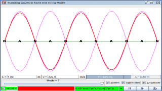
http://physics.bu.edu/~duffy/HTML5/transverse_standing_wave.html
What is the purpose of this simulation model?
This simulation model aims to numerically calculate the vibrations of a stretched string by using a lattice-elasticity model. It allows users to study the string's behavior, first in the low-amplitude limit to verify standard properties, and then to explore the nonlinear properties that emerge as the amplitude of vibration increases.
How does the simulation model represent a continuous string?
The continuous string is modeled as a series of \(N+1\) discrete point masses connected by springs. The two end masses are fixed. The interactions between these masses, governed by Hooke's law springs, approximate the elastic properties of the continuous string. By increasing the number of masses (\(N\)), the model should better approximate the behavior of a real string.
What forces are acting on the masses in the model?
The primary forces acting on each mass (except the fixed ends) are the forces from the two adjacent springs connecting it to its neighbors. These forces are calculated based on Hooke's Law, where the force is proportional to the difference between the current length of the spring and its equilibrium length (\(r_0\)), and directed along the line connecting the two masses.
How are the microscopic properties of the model (m, k, r0) related to the macroscopic properties of the string (M, L, Y, A)?
The microscopic properties are derived from the macroscopic properties to ensure the model accurately represents the string. The mass of each point mass (\(m\)) is the total mass (\(M\)) divided by the number of segments (\(N\)), so \(m = M/N\), or equivalently, \(m = \text{density} \times \text{length} / N\). The equilibrium length (\(r_0\)) of each spring is the unstretched length (\(L\)) divided by \(N\), so \(r_0 = L/N\). The spring constant (\(k\)) is related to the stiffness (\(\gamma = AY\)) and the length, given by \(k = \text{stiffness} \times N / \text{length}\).
What are the initial conditions for a stretched but unexcited string in this model?
For a stretched but unexcited string with endpoints fixed at a distance \(L' > L\), the initial \(y\)-positions (\(y_i\)) and \(y\)-velocities (\(v_{yi}\)) of all the masses would be zero. The initial \(x\)-positions (\(x_i\)) would be distributed uniformly between the fixed endpoints, so \(x_i = i \times (L'/N)\) for \(i\) from 0 to \(N\). The initial \(x\)-velocities (\(v_{xi}\)) would also be zero. This setup represents the string being stretched to a new equilibrium length \(L'\) under tension \(T\), without any initial displacement or velocity in the transverse direction.
How can the period of a normal mode be measured in the simulation?
The period of a normal mode \(n\) can be measured by observing the motion of a mass near an antinode of that mode. If the initial displacement is in the +y direction, one full period is completed when the mass moves down, then back up, and starts to move down again. This can be tracked in the code by monitoring the y-velocity (\(v_y\)) of the chosen mass for a change from positive to negative. The time elapsed between two such changes (separated by a full cycle) represents the period.
How does the amplitude of vibration affect the string's behavior in this model, particularly regarding the ideal wave equation?
The ideal wave equation, which describes noninterfering superpositions of normal modes with amplitude-independent frequencies, is derived using the small-angle approximation. This approximation is only valid when the amplitude of vibration (\(A\)) is very small (\(A \rightarrow 0\)). As the amplitude increases, this approximation breaks down. The simulation, by not relying on this approximation, can reveal nonlinear behaviors such as amplitude-dependent frequencies and the generation of harmonics, which are not predicted by the ideal wave equation.
How does the number of masses (\(N\)) in the model affect the accuracy of the simulation for different normal modes?
The number of masses (\(N\)) influences the model's ability to accurately represent the string's behavior, especially for higher-frequency normal modes. A larger \(N\) provides a finer discretization of the string, allowing the model to better capture the shorter wavelengths associated with high-\(n\) modes. For low-\(n\) normal modes, even a smaller \(N\) might provide a reasonable approximation. However, for accurately modeling the higher harmonics and nonlinear effects that might involve these higher modes, a larger \(N\) is more critical. The computational cost also increases with \(N\).
- Details
- Parent Category: 03 Waves
- Category: 01 General Waves
- Hits: 6081