About
3D function plotter
x = fx( p, q ); y = fy( p, q ); z = fz( p, q)
This function plotter displays animated 3D surfaces described by three coordinate functions of two variables p, q for the spatial coordinates x, y, z.
The coordinate functions fx , fy , fz , which in the simulation are shown in three editable text fields, map the points of the plane pq unambiguously into a surface in space xyz. If fx , fy ,, fz contain periodic functions of the parameters p and q, closed or intersecting surfaces may be produced.
The functions may contain four constants a, b, c, v that can be changed by sliders. In the predefined functions v is used to animate the surfaces by oscillating one or more of the coordinates via time dependent terms.
At the start of the simulation you will see the projection of a plane in space, viewed under perspective distortion. It is embedded into an x y z tripod, and is accompanied by the x y- plane z = 0. This plane can be deactivated by its check box.
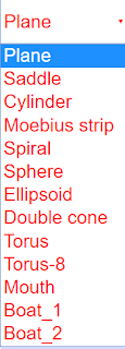
Other predefined surfaces in space can by selected in the ComboBox.
The formula for the plane (pi ≡ π) shows that v modulates the z-function periodically: z = cos(vt)(a - 0.6)p. For t = 0 the modulation factor is 1; a determines the degree of modulation; (a- 0.6) defines a reasonable initial value. The other variable constants b, c are not used with the plane.
Play starts the animation, with time t starting at 0, as indicated in the t number field. With cos(t) fluctuating periodically, the plane oscillates in space. Slider a defines the base orientation. Pause freezes the animation at any spatial position. Reset leads back to the initial conditions.
The range of p and q is ∓ π . Scaling of all three axes x, y, z has a range of ∓ 1. The xy-plane cuts the z axis at the center of the z- arrow. As variables p and q change in the range -π to +π, a periodic function as cos(p) completes a full period in the variable plane.
The orientation of the tripod in space can be changed by drawing with the mouse.
Other ways of visualization are described in the next page.
Predefined functions are selected in the ComboBox with a mouse click. Constants a,b,c can be varied by sliders while the animation is running. By editing the formulas you can change the terms that are animated. You can input new parametric formulas to create your own surfaces. Do not forget to press the ENTER key after a change!
Touching a surface with the mouse pointer lets its color filling disappear; the wire mesh of calculation will be pronouncedly visible.
Visualization alternatives
Rotation: Mark any point within the tripod by the mouse pointer and draw (while the left mouse key stays pressed).
Shift: Draw while the Strg key is pressed.
Zoom: Draw while the Shift key is pressed
Correction: To return to the default projection choose another surface, and then the oldone anew
Show coordinates: Mark a point on the surface while pressing the Alt key. When you draw, a cutting plane will pass through the surface. Depending on orientation, different cuts can be evaluated.
Camera- Inspector: Press the right mouse key. A context menu will appear. Choose Elements option/ drawing 3D panel/ Camera. The Camera Inspector will appear. It will stay visible until it is deactivated. It offers the following options:
Perspective: Distant lines appear shorter than near ones.
No perspective: No perspective distortion.
Planar xy or yz or yx : One looks onto the respective planes.
Other options: Degree and angle of perspective can be defined.
Optimizing parameters. The spatial impression can be optimized by adjusting parameters. The optimum will be different for different projections.
The context menu also offers programs for producing a picture or a video.
Predefined functions
As p and scale in pi (π), for all terms where p and q enter directly into formulas for x ,y, z (e.g not in periodic function of the variables), a factor 1/pi (1/π) appears. A factor cos(v*t) indicates that the associated term is animated. Reset redefines t = 0 and hence cos(vt) = 1.
Fixed numbers in the formulas are used to define a reasonable scaling at the start of the simulation for uniform default values of parameters a, b, c (= 0.5).
x_function = p/pi
y_function = q/pi
z_function = cos(v*t)*(a/pi-0.6)*p
Plane
x_function = p/pi
y_function = q/pi
z_function = cos(v*t)*p*q/pi^2
Saddle
x_function = cos(v*t)*a*cos(p)
y_function = b*sin(p)
z_function = c*q/(2*pi)
Cylinder
x_function = a*cos(p)*(1+q/(2*pi)*cos(p/2))
y_function = 2*b*sin(p)*(1+q/(2*pi)*cos(p/2))
z_function = c*q/(pi)*sin(p/2*t)
Möbius strip
x_function = cos(v*t)*a*cos(p)*abs(cos(q))
y_function = cos(v*t)*a*sin(p)*abs(cos(q))
z_function = cos(v*t)*a*sin(q)
Sphere
x_function = a*cos(p)*abs(cos(q))
y_function = cos(v*t)*b*sin(p)*abs(cos(q))
z_function = c*sin(q)
Ellipsoid
x_functio n= a/pi*q*cos(p)*cos(v*t)");
y_function = b/pi*q*sin(p)*cos(v*t)");
z_function = c*q/pi");
Double cone
x_function = (a+0.6*cos(v*t)*b*cos(q))*sin(p)
y_function = (c+0.6*cos(v*t)*b*cos(q))*cos(p)
z_function = 0.6*b*sin(q)
Torus
x_function = 2*(a+0.3*b*cos(q))*sin(p)*cos(p)
y_function = 2*((cos(v*t)^2)*c+0.3*b*cos(q))*cos(p)*cos(p)*cos(p)
z_function = 0.6*b*sin(q)
Torus-8
x_function = (cos(v*t)*c+0.3*b*cos(q))*cos(p)*cos(p)*cos(p)
y_function = (a+0.3*b*cos(q))*sin(p)
z_function = b*0.3*sin(q)
Mouth
x_function = (0.4*c+0.4*b*cos(q))*cos(p)*cos(p)*cos(p)
y_function = (2*a+0.4*b*cos(q))*sin(p)
z_function = cos(v*t)*0.4*b*cos(q)
Boat_1
x_function = (0.4*c+0.4*b*cos(q))*cos(p)*cos(p)*cos(p)
y_function = (2*a+0.4*b*cos(q))*sin(p)
z_function = cos(v*t)*0.4*b*cos(q)*cos(q)
Boat_2
E1: Test the different surfaces without a change of parameters. Rotate the frames and train your 3D perception of these functions.
E2: Study the formulas and develop a sense for the relation between formulas and surface.
E3: Rotate, tilt and zoom the 3D projection to optimize the visual impression of the surface . Use the Camera Inspector, too (see Visualization page).
E4: Vary parameters and study the influence on the appearance of the surface.
E5: Change signs (+/-) in the formulas and study the effect.
E6: Vary the grade of power functions in the formulas and study the resulting surfaces.
E7: Edit the formulas freehandedly and consider in advance how that should influence the surface.
E8: Animate different parameters, or two at the same time.
E9: Delete the animation term and use p as a free fourth parameter in your own formula.
E10: Reflect in using 3D surfaces created this way in design of 3D objects. The last three predefined functions are intended as encouragement (mouth and boat). Remember that numerical machines could directly use the formulas for control.
Translations
| Code | Language | Translator | Run | |
|---|---|---|---|---|
 |
||||
Credits
 Dieter Roess - WEH- Foundation; Fremont Teng; Loo Kang Wee
1. Overview:
This document provides a briefing on the "Parametric Surface 3D Simulator JavaScript Simulation Applet HTML5," an interactive resource hosted by Open Educational Resources / Open Source Physics @ Singapore. This simulation is a tool for learning and teaching mathematics, specifically the visualization of 3D surfaces defined by parametric equations. It allows users to explore how changing the parameters of these equations affects the resulting shapes in a dynamic and interactive environment.
2. Main Themes and Important Ideas:
- Parametric Representation of 3D Surfaces: The core concept is the representation of a 3D surface using three coordinate functions (x, y, z) that depend on two parameters, typically denoted as p and q. The simulator emphasizes this relationship: "x = fx( p, q ); y = fy( p, q ); z = fz ( p, q)." This allows for the generation of complex and varied surfaces.
- Interactive Exploration and Visualization: The applet provides a highly interactive environment for users to manipulate and observe these surfaces. Key features include:
- Dynamic Adjustment of Parameters: Sliders control four constants (a, b, c, v) that influence the coordinate functions. "The functions may contain four constants a, b, c, v that can be changed by sliders."
- Animation: The constant v is often used to animate surfaces over time, introducing a dynamic element to the visualization. "In the predefined functions v is used to animate the surfaces by oscillating one or more of the coordinates via time dependent terms."
- Predefined Surface Examples: A ComboBox offers a selection of predefined parametric surfaces, such as a plane, saddle, cylinder, Möbius strip, sphere, ellipsoid, double cone, and various torus shapes. These serve as starting points for exploration.
- User-Defined Functions: Users can directly edit the formulas for the x, y, and z coordinates to create their own unique surfaces. "By editing the formulas you can change the terms that are animated. You can input new parametric formulas to create your own surfaces. Do not forget to press the ENTER key after a change!"
- Interactive Manipulation of the 3D View: Users can rotate, shift, and zoom the 3D projection using mouse controls and modifier keys (Strg, Shift). "Rotation: Mark any point within the tripod by the mouse pointer and draw (while the left mouse key stays pressed). Shift: Draw while the Strg key is pressed. Zoom: Draw while the Shiftkey is pressed."
- Camera Inspector: A right-click menu provides access to a "Camera Inspector" with options to control perspective (perspective, no perspective, planar views) and optimize parameters for different projections.
- Visualization Alternatives: Other features include the ability to show coordinates by pressing Alt and drawing, which creates a cutting plane through the surface. Touching the surface with the mouse reveals the underlying wire mesh.
- Learning and Teaching Mathematics: The simulator is explicitly designed for educational purposes, aiming to enhance the understanding of parametric equations and their geometric representations. The inclusion of predefined examples and the ability to create custom surfaces encourages experimentation and deeper learning. The "Sample Learning Goals" section (though the text is empty in this excerpt) further reinforces this objective.
- Practical Applications: One of the "experiments" (E10) prompts reflection on the use of these 3D surfaces in the "design of 3D objects," highlighting a potential connection to real-world applications and the use of numerical machines for control based on these formulas.
- Technical Implementation: The applet is a "JavaScript Simulation Applet HTML5," indicating its web-based nature and reliance on these technologies for interactive functionality. The embedding code provided allows for easy integration into other webpages.
3. Predefined Functions and Their Characteristics:
The document lists several predefined functions, illustrating the variety of surfaces that can be generated. Key features within the formulas include:
- Parameters p and q: These are the independent variables that define the surface. Their range is typically ∓ π.
- Constants a, b, c, v: These constants can be manipulated by sliders to alter the shape and animation of the surfaces.
- Animation Term cos(vt)*: This term introduces time dependence, causing the surface to oscillate or change dynamically when the "Play" button is activated. "A factor cos(vt) indicates that the associated term is animated. Reset redefines t = 0 and hence cos(vt) = 1.*"
- Scaling Factor 1/pi: This factor appears in terms where p and q are directly used (not within periodic functions), likely to normalize the effect of the parameter range. "As p and scale in pi (π), for all terms where p and q enter directly into formulas for x ,y, z (e.g not in periodic function of the variables), a factor 1/pi (1/π) appears."
Examples of Predefined Functions (Illustrative):
- Plane: Demonstrates a simple linear relationship between the parameters and the coordinates, with animation affecting the z-coordinate. "*z_function = cos(vt)*(a/pi-0.6)p"
- Saddle: Shows a more complex relationship, with the z-coordinate being a product of p and q, also animated. "z_function = cos(v*t)pq/pi^2"
- Sphere: Uses trigonometric functions of p and q to create a closed, spherical surface, with animation potentially affecting scaling or position.
- Möbius strip: A classic example of a non-orientable surface generated through specific parametric equations.
4. Instructions for Use:
The document provides basic instructions for interacting with the simulator:
- Object Combo Box: Selects different predefined shapes.
- Sliders: Modify the constants a, b, c.
- Analytical Surface Equation Boxes: Allow users to input custom formulas.
- Show xy-plane Check Box: Toggles the visibility of the z=0 plane.
- Toggling Full Screen: Double-click to enter/exit full-screen mode (when not playing).
- Play/Pause and Reset Buttons: Control the animation and revert to initial conditions.
5. Suggested Experiments:
A list of suggested experiments encourages users to actively engage with the simulator and explore the relationship between the equations and the resulting surfaces. These experiments range from simple observation to advanced formula editing and reflection on applications.
6. Credits and Licensing:
The simulator is credited to Dieter Roess, Fremont Teng, and Loo Kang Wee. The content is licensed under the Creative Commons Attribution-Share Alike 4.0 Singapore License, with a separate license and contact information provided for commercial use of the EasyJavaScriptSimulations Library.
7. Related Resources:
The document includes a long list of other interactive simulations available on the platform, covering various topics in physics and mathematics. This indicates a rich collection of open educational resources.
8. Conclusion:
The "Parametric Surface 3D Simulator JavaScript Simulation Applet HTML5" is a valuable interactive tool for learning and teaching the concept of parametric surfaces in three dimensions. Its user-friendly interface, predefined examples, customization options, and interactive visualization features make it an effective resource for students and educators seeking a dynamic and engaging way to explore mathematical concepts. The emphasis on experimentation and the connection to potential real-world applications further enhance its educational value.
Parametric Surface 3D Simulator Study Guide
Quiz
- What is the fundamental purpose of the Parametric Surface 3D Simulator?
- Explain how the coordinate functions fx, fy, and fz define a 3D surface within the simulator.
- How do the constants a, b, c, and v influence the displayed parametric surfaces?
- Describe the effect of activating the "Play" button in the simulation. What role does the variable 't' play?
- What is the range of values for the parameters p and q in the simulator? What is the scaling range for the x, y, and z axes?
- List three interactive visualization techniques available in the simulator and briefly describe how to use them.
- What is the purpose of the "Camera Inspector" and what are two options it provides for altering the view of the 3D surface?
- Explain the significance of the term "cos(v*t)" appearing in the predefined function formulas. What does the "Reset" button do in relation to this term?
- Describe how you can load and interact with one of the predefined surface functions within the simulator.
- What is the purpose of the "Experiments" section provided in the source material? Give an example of one suggested experiment.
Quiz Answer Key
- The Parametric Surface 3D Simulator allows users to visualize and interact with three-dimensional surfaces that are mathematically defined by parametric equations. It plots these surfaces based on three coordinate functions of two variables, p and q, mapping a 2D plane to a 3D space.
- The coordinate functions fx(p, q), fy(p, q), and fz(p, q) determine the x, y, and z coordinates of each point on the 3D surface based on the input values of the two parameters, p and q. As p and q vary within their defined ranges, these functions generate the spatial coordinates that form the surface.
- The constants a, b, c, and v are adjustable parameters that can modify the shape, size, position, and animation of the parametric surfaces. Sliders control the values of these constants, allowing users to dynamically observe their impact on the surface defined by the parametric equations. The constant 'v' is specifically used to introduce time-dependent oscillations for animation.
- Activating the "Play" button starts the animation of the surface, with the variable 't' representing time, beginning at 0. The term "cos(t)" or variations like "cos(v*t)" in the function formulas cause the surface coordinates to fluctuate periodically as time progresses, resulting in the visual oscillation of the surface.
- The range of values for both parameters p and q is from -π to +π. The scaling of all three spatial axes (x, y, and z) has a range of -1 to +1, defining the boundaries of the viewing space for the generated surfaces.
- Three interactive visualization techniques are: Rotation, achieved by clicking and dragging the mouse within the tripod frame to change the viewing angle; Zoom, performed by pressing the Shift key while clicking and dragging the mouse to magnify or reduce the size of the displayed surface; and Shift, done by pressing the Strg key while clicking and dragging to translate the surface within the viewing area.
- The "Camera Inspector" is a tool accessed via the right-click context menu that allows users to adjust the projection and viewing parameters of the 3D scene. Two options provided are Perspective, which simulates how distant objects appear smaller, and No perspective, which eliminates this depth distortion, rendering parallel lines as parallel in the projection.
- The factor "cos(v*t)" in the formulas indicates that the associated term will oscillate over time, creating an animated effect on the surface. The "Reset" button redefines the time variable 't' to 0, which sets the value of "cos(v*t)" back to 1, returning the animation to its initial state.
- To load a predefined function, click on the ComboBox and select the desired surface (e.g., Plane, Saddle, Cylinder). The simulator will then display the corresponding parametric equations and the resulting 3D shape. Users can then interact with the sliders to change the constants and observe the dynamic modifications to the selected surface.
- The "Experiments" section suggests various ways for users to explore and understand the relationship between the parametric equations and the generated 3D surfaces through interactive manipulation. For example, E1 suggests testing the different surfaces without changing parameters to develop 3D perception.
Essay Format Questions
- Discuss the relationship between the mathematical representation of parametric surfaces (coordinate functions and parameters) and their visual manifestation in the 3D simulator. How does manipulating the equations and parameters affect the geometry of the displayed shapes?
- Analyze the role of interactivity in the Parametric Surface 3D Simulator as a tool for learning and teaching mathematics. How do the different visualization and manipulation features contribute to a deeper understanding of parametric equations and 3D geometry?
- Compare and contrast the different predefined parametric surfaces provided in the simulator. Discuss how their respective mathematical formulas lead to their unique geometric characteristics and how animation can further illustrate their properties.
- Evaluate the potential applications of understanding and manipulating parametric surfaces in various fields, such as computer graphics, design, and scientific visualization. How might a tool like this simulator aid in these areas?
- Describe the process of creating a new parametric surface within the simulator by editing the formulas. What considerations should a user take into account when defining their own coordinate functions to achieve a desired 3D shape and potentially animate it?
Glossary of Key Terms
- Parametric Surface: A three-dimensional surface defined by a set of parametric equations, where the coordinates (x, y, z) of points on the surface are expressed as functions of two independent parameters (typically denoted as p and q).
- Coordinate Functions (fx, fy, fz): The mathematical functions that define the x, y, and z coordinates of points on a parametric surface in terms of the parameters p and q.
- Parameters (p, q): Independent variables that serve as inputs to the coordinate functions, determining the location of points on the parametric surface. In this simulator, their range is typically -π to +π.
- Constants (a, b, c, v): Adjustable numerical values within the coordinate functions that control the shape, size, orientation, and animation of the parametric surface.
- Animation: The dynamic change of a surface over time, often achieved by incorporating a time-dependent term (in this case, involving the constant 'v' and time 't') into the coordinate functions, causing the surface to oscillate or morph.
- Tripod: The three mutually perpendicular axes (x, y, z) displayed in the simulator, providing a spatial frame of reference for the plotted parametric surfaces.
- xy-plane (z = 0): A flat plane in the 3D space where the z-coordinate is always zero. The simulator displays this plane as a visual aid for spatial orientation.
- ComboBox: A drop-down menu in the simulator's interface that allows users to select from a list of predefined parametric surfaces.
- Sliders: Interactive graphical elements that enable users to continuously adjust the values of the constants (a, b, c, v), allowing for real-time observation of their effect on the surface.
- Perspective Distortion: A visual effect that makes distant objects appear smaller than objects closer to the viewer, contributing to a sense of depth in the 3D rendering. The Camera Inspector allows toggling this effect.
Sample Learning Goals
[text]
For Teachers
Parametric Surface 3D Simulator JavaScript Simulation Applet HTML5
Instructions
Object Combo Box
Sliders
Analytical Surface Equation Boxes
Show xy-plane Check Box
Toggling Full Screen
Play/Pause and Reset Buttons
Research
[text]
Video
[text]
Version:
Other Resources
[text]
Frequently Asked Questions: Parametric Surface 3D Simulator
What is the Parametric Surface 3D Simulator?
The Parametric Surface 3D Simulator is an interactive JavaScript application that visualizes three-dimensional surfaces defined by parametric equations. These equations express the spatial coordinates (x, y, z) as functions of two independent parameters, typically denoted as p and q. The simulator allows users to explore and manipulate these surfaces in real-time.
How are surfaces defined in the simulator?
Surfaces are defined by three coordinate functions: x = fx(p, q), y = fy(p, q), and z = fz(p, q). These functions are entered into editable text fields within the simulator. The parameters p and q typically range from -π to +π, and they map points on a 2D plane to a 3D surface in the xyz-space. The functions can include mathematical operations, constants (a, b, c, v), and periodic functions, enabling the creation of a wide variety of surface shapes, including closed or intersecting ones.
What are the constants a, b, c, and v used for?
The coordinate functions can incorporate four adjustable constants: a, b, c, and v. These constants can be modified using sliders within the simulator, allowing users to dynamically change the properties and appearance of the generated surfaces. The constant v is often used in conjunction with time-dependent terms (e.g., cos(vt)) to animate the surfaces by oscillating one or more of the coordinates.
How can I interact with the 3D surfaces in the simulator?
The simulator offers several ways to interact with the visualized surfaces:
- Rotation: Click and drag the mouse within the tripod frame to rotate the 3D view.
- Shift: Press and hold the "Strg" key while dragging the mouse to shift the view.
- Zoom: Press and hold the "Shift" key while dragging the mouse to zoom in or out.
- Camera Inspector: Right-click within the tripod to access a context menu and open the Camera Inspector. This tool allows you to toggle perspective, choose planar views (xy, yz, zx), and adjust the degree and angle of perspective.
- Show Coordinates/Cutting Plane: Press and hold the "Alt" key while clicking on the surface. Dragging the mouse will then introduce a cutting plane through the surface, revealing different cross-sections depending on the orientation.
What are the "Predefined functions" and how can I use them?
The simulator includes a selection of "Predefined functions" that represent various mathematical surfaces like a plane, saddle, cylinder, Möbius strip, sphere, ellipsoid, double cone, torus, and more. These can be accessed and displayed by selecting them from the "ComboBox." Once a predefined function is selected, you can observe its shape and further modify it using the sliders for the constants a, b, and c, or by editing the formulas directly.
How can I create and animate my own surfaces?
To create your own surfaces, you can edit the formulas in the x_function, y_function, and z_function text fields. After making changes, press the "ENTER" key to apply them. To animate a surface, incorporate the constant v with a time-dependent function like cos(v*t) into one or more of the coordinate functions. The "Play" button starts the animation, and the "Pause" and "Reset" buttons allow you to control the animation's state.
What are the "Experiments" suggested in the simulator?
The "Experiments" section provides a series of guided explorations to help users understand the relationship between the parametric equations and the resulting 3D surfaces. These experiments encourage users to:
- Observe predefined surfaces.
- Study the formulas and their connection to the shapes.
- Practice visualization techniques (rotation, tilt, zoom).
- Investigate the impact of changing parameters and signs in the formulas.
- Experiment with power functions and freehand formula editing.
- Animate parameters.
- Explore using p as a fourth parameter.
- Reflect on the application of these surfaces in 3D object design.
Is this simulator open educational resource?
Yes, the Parametric Surface 3D Simulator is provided as an Open Educational Resource (OER) under the Open Source Physics @ Singapore initiative. The content is licensed under the Creative Commons Attribution-Share Alike 4.0 Singapore License, promoting free use and adaptation for educational purposes. The underlying EasyJavaScriptSimulations Library may have separate commercial use terms as specified in the provided link.
- Details
- Written by Fremont
- Parent Category: Interactive Resources
- Category: Mathematics
- Hits: 5544


.png
)
