About

For Teachers

- PendulumSwingModelHannah1.mp4

Credits

Author: video: hannah tan, model: lookang

Document Brief: Modeling Pendulum Swing Dynamics Using Tracker

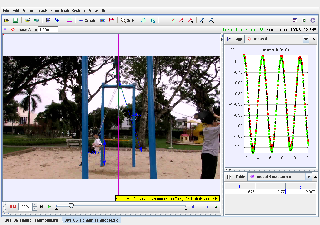
This document explores the dynamics of a pendulum swing using Tracker’s modeling capabilities. The motion is described using polar coordinates and modeled with force functions representing angular motion, including damping effects. Key parameters such as mass ($m$), gravity ($g$), length ($r$), and damping constant ($k$) are incorporated into the model.

Purpose:

To analyze the pendulum swing dynamics, including angular displacement, angular velocity, and damping effects, using Tracker’s Model Builder.

Key Features:

• Motion tracked in polar coordinates ($\theta ,r$).
• Force functions applied to model angular motion:
  • Restoring force: Fθ=−m⋅g⋅cos⁡(θ)−k⋅ω⋅rF_\theta = -m \cdot g \cdot \cos(\theta) - k \cdot \omega \cdot rFθ​=−m⋅g⋅cos(θ)−k⋅ω⋅r.
  • Radial force: Fr=−m⋅r⋅ω2F_r = -m \cdot r \cdot \omega^2Fr​=−m⋅r⋅ω2.
• Graphical analysis of angular displacement ($\theta$) vs. time ($t$).

Study Guide: Modeling Pendulum Swing with Tracker

Learning Objectives:

1. Understand the forces acting on a pendulum swing in polar coordinates.
2. Analyze the effects of gravity and damping on the pendulum’s angular motion.
3. Validate the modeled motion against experimental data.

Step-by-Step Guide:

1. Setup and Calibration:

   • Import the pendulum swing video into Tracker.
   • Calibrate the scale using visible reference objects and define the coordinate system in polar form.

2. Tracker Motion Tracking:

   • Track the pendulum bob’s position frame by frame.
   • Record angular displacement ($\theta$) and length ($r$) data.

3. Modeling with Force Functions:

   • Open the Model Builder in Tracker.
   • Define parameters and initial values:
     • $m=1.0$ kg (mass).
     • $g=9.81$ m/s2^22 (gravitational acceleration).
     • $k=0.02$ (damping constant).
     • Initial conditions: θ0=67∘\theta_0 = 67^\circθ0​=67∘, ω0=−4.11∘/s\omega_0 = -4.11^\circ/\text{s}ω0​=−4.11∘/s.
   • Apply force functions:
     • Fθ=−m⋅g⋅cos⁡(θ)−k⋅ω⋅rF_\theta = -m \cdot g \cdot \cos(\theta) - k \cdot \omega \cdot rFθ​=−m⋅g⋅cos(θ)−k⋅ω⋅r.
     • Fr=−m⋅r⋅ω2F_r = -m \cdot r \cdot \omega^2Fr​=−m⋅r⋅ω2.

4. Graphical Analysis:

   • Plot angular displacement ($\theta$) vs. time ($t$):
     • Observe periodic oscillations and damping effects.
   • Analyze angular velocity ($\omega$) for phase relationships with displacement.

5. Applications:

   • Use the model to study real-world damping effects in mechanical systems.
   • Apply insights to pendulum-based systems like playground swings or seismometers.

Tips for Success:

• Ensure accurate tracking of the pendulum’s motion for reliable modeling results.
• Use small initial angles (θ<15∘\theta < 15^\circθ<15∘) for SHM approximation, but the model handles larger angles with damping.

FAQ: Pendulum Swing Model in Tracker

1. Why use polar coordinates for this model?

Polar coordinates ($r,\theta$) simplify the analysis of rotational motion, aligning with the pendulum’s natural movement.

2. What is the role of the damping constant ($k$)?

The damping constant ($k$) represents energy loss due to air resistance or friction, which reduces the pendulum’s amplitude over time.

3. How do force functions describe the motion?

• Fθ=−m⋅g⋅cos⁡(θ)−k⋅ω⋅rF_\theta = -m \cdot g \cdot \cos(\theta) - k \cdot \omega \cdot rFθ​=−m⋅g⋅cos(θ)−k⋅ω⋅r: Restoring force due to gravity and damping.
• Fr=−m⋅r⋅ω2F_r = -m \cdot r \cdot \omega^2Fr​=−m⋅r⋅ω2: Centripetal force due to rotational motion.

4. Why is angular displacement ($\theta$) sinusoidal?

For small angles, the restoring force approximates SHM, resulting in sinusoidal angular displacement.

5. Can this model handle large angles?

Yes, the model incorporates non-linear terms, allowing analysis of larger angular displacements.

6. How is damping observed in the graph?

Damping is visible as a gradual decrease in the oscillation amplitude over time in the angular displacement ($\theta$) vs. time graph.

7. What are the practical applications of this model?

• Understanding playground swing dynamics.
• Designing pendulum-based systems like clocks or oscillators.
• Analyzing damping effects in engineering systems.