{source}
<?php  require_once JPATH_SITE.'/TTcustom/TT_contentparser.php';$parameters = array("topicname" => "math/Fields_Vector", "modelname" => "ejss_model_e_Vectorfield_2D");echo generateSimHTML($parameters, "EJSS");
?>
{/source}
Sample Learning Goals
[text]
For Teachers
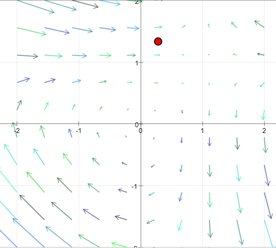
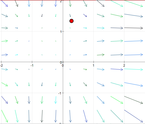
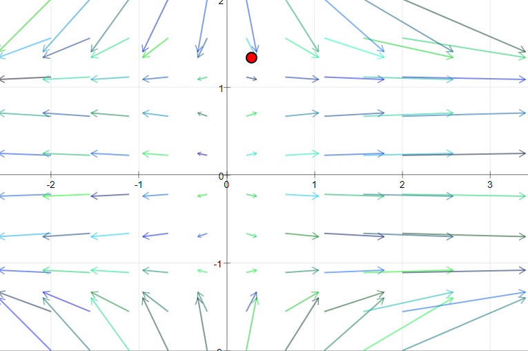
Two Dimensional Vector Fields JavaScript Simulation Applet HTML5
Instructions
Function Combo Box
Arrow Size Slider
Draggable Red Ball

Toggling Full Screen
Play/Pause and Reset Buttons

Research
[text]
Video
[text]
Version:
Other Resources
[text]
Frequently Asked Questions: Two Dimensional Vector Fields Simulation
What is a two-dimensional vector field as shown in this simulation?
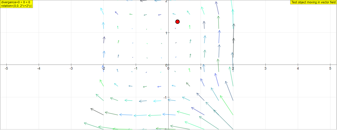
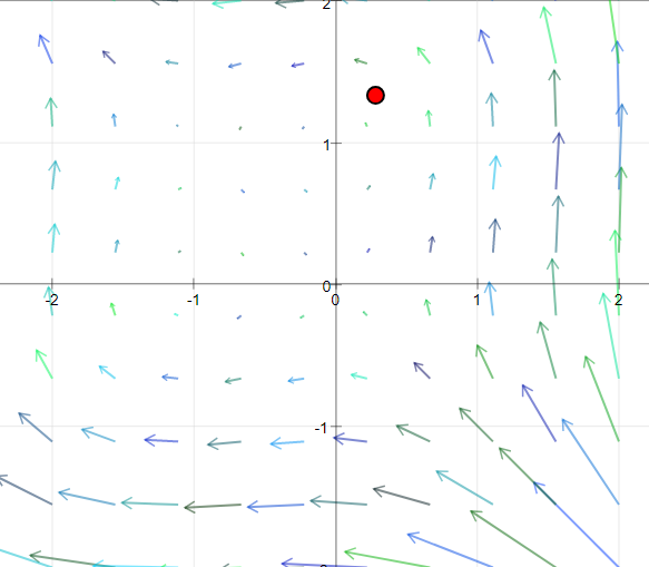
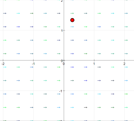
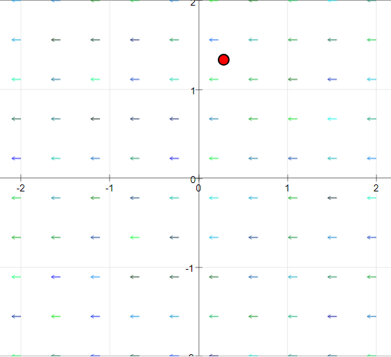
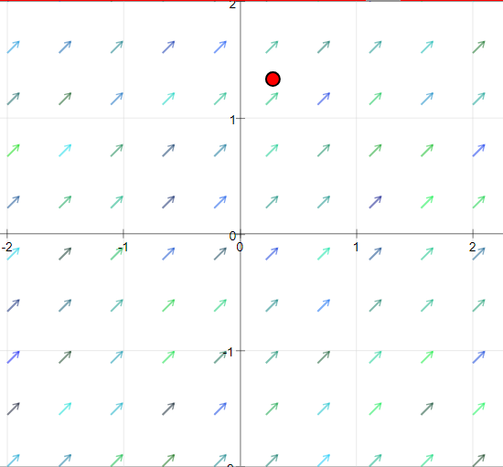
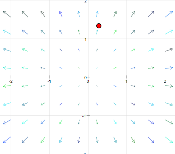
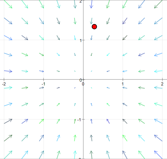
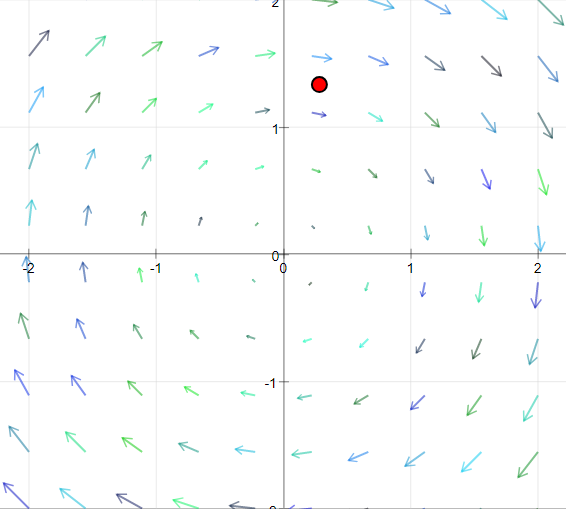
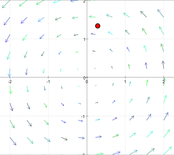
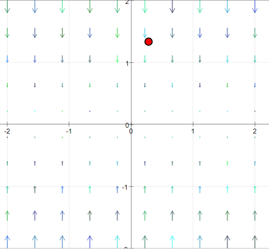
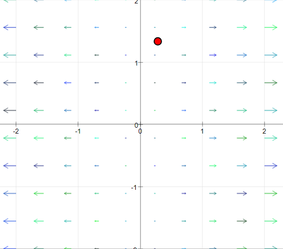
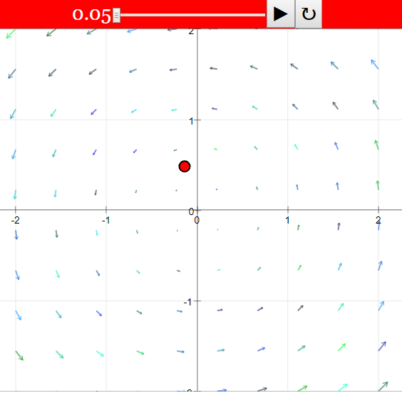
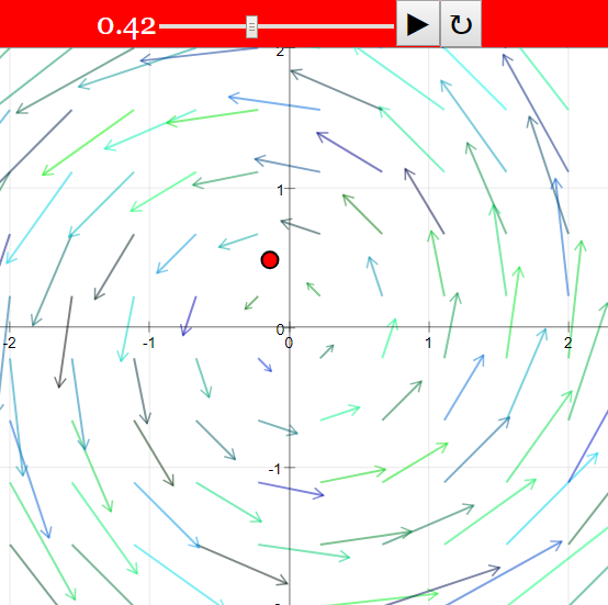
This simulation visualizes a two-dimensional vector field, which can be thought of as representing the xy-cross section of a three-dimensional field that remains constant in the z direction (similar to an infinitely long cylinder). It displays flow fields where each point in the xy-plane is associated with a velocity vector having components in the x ($a_x$) and y ($a_y$) directions. The direction of the flow is indicated by arrows of uniform length, while the magnitude (size) of the vector is represented by color gradation.
What can I observe and learn from this simulation?
You can observe various predefined vector fields, such as those with vortices, constant flows, or radial patterns. By examining the arrows and the movement of a red test object, you can gain an intuitive understanding of the field's direction and magnitude at different locations. The simulation also allows you to see the mathematical formulas for the vector components, the divergence (source/sink strength), and the z-component of the rotation (vorticity) of the field. This helps connect the visual representation to the underlying mathematical concepts.
How can I interact with the simulation?
The simulation offers several interactive features. You can select from various predefined vector fields using a combobox. You can also directly edit the formulas for the x and y components of the vector field in the white text fields and observe the resulting changes. A red test object can be started to follow the flow, stepped forward incrementally, or dragged with the mouse to explore the field. Sliders allow you to adjust the zoom level (scale of coordinates) and the arrow length. Buttons are available to start/pause the motion, perform a single step, reset all parameters to their initial values, and reset the point to its starting position.
What is divergence and rotation in the context of this 2D vector field?
Divergence ($\nabla \cdot \mathbf{a} = \frac{\partial a_x}{\partial x} + \frac{\partial a_y}{\partial y}$) in this simulation indicates the source or sink strength of the vector field at a given point. A positive divergence suggests a source (flow emanating outwards), while a negative divergence suggests a sink (flow converging inwards). The rotation (curl in 2D, specifically the z-component $\frac{\partial a_y}{\partial x} - \frac{\partial a_x}{\partial y}$) indicates the local rotational tendency or vorticity of the field. A non-zero rotation implies the presence of vortices or swirling motion.
When is a vector field considered "without vortex" or "without source"?
A vector field is without vortex (irrotational) when its rotation is zero ($\frac{\partial a_y}{\partial x} - \frac{\partial a_x}{\partial y} = 0$). This condition is satisfied if the x-component ($a_x$) is solely a function of x, and the y-component ($a_y$) is solely a function of y. A field is without source (incompressible or solenoidal) when its divergence is zero ($\frac{\partial a_x}{\partial x} + \frac{\partial a_y}{\partial y} = 0$). This requires that the partial derivatives of the components with respect to their corresponding coordinates are equal in magnitude but opposite in sign.
How does the red test object move, and what can I learn from its movement?
When the start button is activated, the red test object moves according to the local velocity vector at its current position. Its movement is governed by the differential equations $\frac{dx}{dt} = a_x$ and $\frac{dy}{dt} = a_y$. By observing the path and speed of the test object, you can qualitatively understand the direction and magnitude of the vector field in different regions. Dragging the object allows you to probe the field at various points and see how the flow would affect a particle placed there.
Can I create and analyze my own vector fields using this simulation?
Yes, the simulation allows you to create your own vector fields. You can select the empty case in the combobox or edit the formulas in the $a_x$ and $a_y$ text fields. After entering your formulas and pressing Enter, the simulation will display the corresponding vector field. You can then calculate the divergence and rotation of your field using partial derivatives and observe its characteristics using the test object and other interactive tools.
Why are divergences sometimes not quoted for linear fields, and what causes acceleration of the test object?
Divergences might not be explicitly quoted for fields with linear components because they can sometimes lead to localized limits or singularities at "sources" or "sinks." The acceleration of the test object occurs when the velocity components $a_x$ and $a_y$ are not constant but change with position ($x$ and $y$). According to the governing differential equations, the rate of change of velocity (acceleration) depends on how the vector components themselves vary across the field. For example, if $a_x$ depends on $x$, then $\frac{da_x}{dt} = \frac{\partial a_x}{\partial x} \frac{dx}{dt} = \frac{\partial a_x}{\partial x} a_x$, indicating acceleration in the x direction if $\frac{\partial a_x}{\partial x} \neq 0$.